
Attractor dynamics
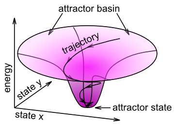
Figure 1: Illustration of attractor dynamics, in terms of a “gravity well”. In the familiar gravity wells that suck in coins at science museums, the attractor state is the bottom hole in the well, where the coin inevitably ends up. This same dynamic can operate in more abstract cases inside bidirectionally connected networks. For example, the x and y axes in this diagram could represent the activities of two different neurons, and the attractor state indicates that the network connectivity prefers to have neuron x highly active, while neuron y is weakly active. The attractor basin indicates that regardless of what configuration of activations these two neurons start in, they’ll end up in this same overall attractor state.
The overall process of converging on a good internal representation given a noisy, weak or otherwise ambiguous input can be summarized in terms of attractor dynamics (Figure 1). An attractor is a concept from dynamical systems theory, representing a stable configuration that a dynamical system will tend to gravitate toward. A familiar example of attractor dynamics is the coin gravity well, often found in science museums. You roll your coin down a slot at the top of the device, and it rolls out around the rim of an upside-down bell-shaped “gravity well”. It keeps orbiting around the central hole of this well, but every revolution brings it closer to the “attractor” state in the middle. No matter where you start your coin, it will always get sucked into the same final state.
This is the key idea behind an attractor: many different inputs all get sucked into the same final state. If the attractor dynamic is successful, then this final state should be the correct categorization of the input pattern. Probably the best subjective experience of this attractor dynamic is when viewing an Autostereogram (wikipedia link) — you just stare at this random-looking pattern with your eyes crossed, until slowly your brain starts to fall into the 3D attractor, and the image slowly emerges. The underlying image contains many individual matches of the random patterns between the two eyes at different lateral offsets — these are the constraints in the multiple constraint satisfaction problem that eventually work together to cause the 3D image to appear — this 3D image is the one that best satisfies all those constraints.
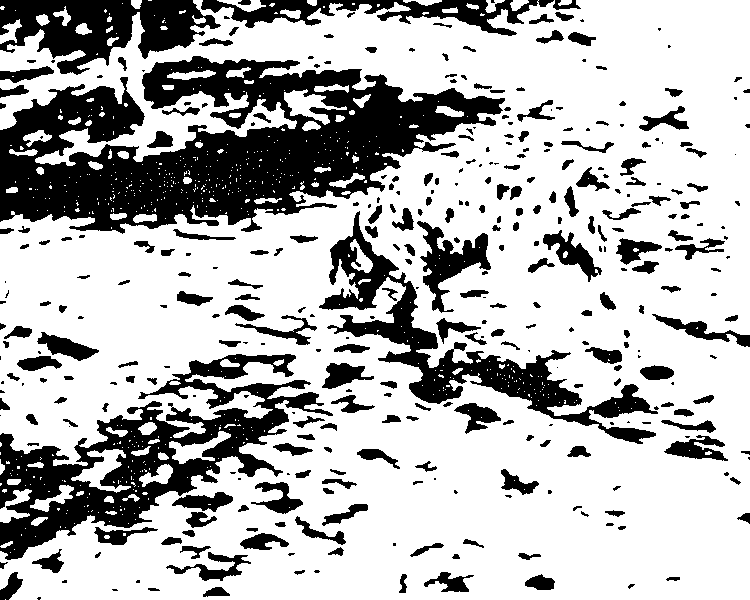
Figure 2: A well-known example of an image that is highly ambiguous, but we can figure out what is going on if an appropriate high-level cue is provided, e.g., “Dalmatian”. This process of top-down knowledge helping resolve bottom-up ambiguity is a great example of bidirectional processing.
There are many different instances where bidirectional excitatory dynamics are evident:
• Top-down imagery — I can ask you to imagine what a purple hippopotamus looks like, and you can probably do it pretty well, even if you’ve never seen one before. Via top-down excitatory connections, high-level verbal inputs can drive corresponding visual representations. For example, imagining the locations of different things in your home or apartment produces reaction times that mirror the actual spatial distances between those objects — we seem to be using a real spatial/visual representation in our imagery.
• Top-down ambiguity resolution — Many stimuli are ambiguous without further top-down constraints. For example, if you’ve never seen Figure 2 before, you probably won’t be able to find the Dalmatian dog in it. But now that you’ve read that clue, your top-down semantic knowledge about what a dalmatian looks like can help your attractor dynamics converge on a coherent view of the scene.
• Pattern completion — If I ask you “what did you have for dinner last night”, this partial input cue can partially excite the appropriate memory representation in your brain (likely in the hippocampus), but you need a bidirectional excitatory dynamic to enable this partial excitation to reverberate through the memory circuits and fill in the missing parts of the full memory trace. This reverberatory process is just like the coin orbiting around the gravity well — different neurons get activated and inhibited as the system “orbits” around the correct memory trace, eventually converging on the full correct memory trace (or not!). Sometimes, in so-called tip of the tongue states, the memory you’re trying to retrieve is just beyond grasp, and the system cannot quite converge into its attractor state. Man, that can be frustrating! Usually you try everything to get into that final attractor. We don’t like to be in an unresolved state for very long.
Energy and Harmony
There is a mathematical way to capture something like the vertical axis in the attractor (Figure 1), which in the physical terms of a gravity well is potential energy. Perhaps not surprisingly, this measure is called energy and it was developed by a physicist named John Hopfield. He showed that local updating of unit activation states ends up reducing a global energy measure, much in the same way that local motion of the coin in the gravity well reduces its overall potential energy (Hopfield, 1982; Hopfield, 1984).
Another physicist, Paul Smolensky, developed an alternative framework with the sign reversed, where local updating of unit activation states increases global Harmony (Smolensky, 1986). That sounds nicer, doesn’t it? We don’t actually need these equations to run our models, and the basic intuition for what they tell us is captured by the notion of an attractor, but the equations are developed below for those who might be interested.
The Hopfield energy equation is:
\[ E = - \frac{1}{2} \sum_j \sum_i x_i w_{ij} y_j \]
where x and y represent the sending and receiving unit activations (indexed by i and j), respectively, and w is the weight between them.
Harmony is literally the same thing without the minus sign:
\[ H = \frac{1}{2} \sum_j \sum_i x_i w_{ij} y_j \]
You can see that Harmony is maximized to the extent that, for each pair of sending and receiving units, the activations of these units \(x_i\) and \(y_j\) are consistent with the weight between these two units. If the weight is large and positive, the network is configured such that it is harmonious if these two units are both active together. If the weight is negative (a simple version of inhibitory projections), then those units contribute to greater harmony only if they have opposite sign (one is active and the other not active).
A key feature of these equations is that local updates drive reliable global effects on energy or Harmony (decreasing the energy or increasing Harmony). To see this, we can use the mathematics of calculus to take the derivative of the global equation with respect to changes in the receiving unit’s activation:
\[ \frac{\partial H}{ \partial y_j} = \sum_i x_i w_{ij} \]
Taking the derivative allows us to find the maximum of a function, which occurs when the derivative is zero. So, this gives us a prescriptive formula for deciding how \(y_j\) should be changed (updated) as a function of inputs and weights so as to maximize Harmony. You might recognize this equation as essentially the net excitatory conductance or net input to a neuron.
This means that updating units with a linear activation function (where activation y = net input directly) would serve to maximize Harmony or minimize energy. Interestingly, a non-linear activation function such as a sigmoid or logistic with a saturating nonlinearity can be derived by introducing an additional “penalty” term (called entropy in the Hopfield framework, and stress in the Smolensky one), that essentially drives the saturation of the neural activation function for high or low values of net input.
Simulations
• faces simulation (Part II) demonstrates how top-down and bottom-up processing interact to produce imagery and help resolve ambiguous inputs (partially occluded faces).
• necker cube simulation demonstrates how lateral excitatory connections can produce attractor dynamics in the case of a classic ambiguous visual stimulus.
• cats and dogs simulation demonstrates bottom-up and top-down dynamics in a semantic network representing different levels of information about cats and dogs.