Reservoir computing

Reservoir computing refers to a family of different algorithms that combine a dynamic network that evolves its state in complex ways over time (the “reservoir”) with a simple layer of output neurons that learn to map this temporally evolving state into relevant target outputs (Figure 1; Maass et al., 2002; Jaeger & Haas, 2004; Verstraeten et al., 2007; Tanaka et al., 2019).

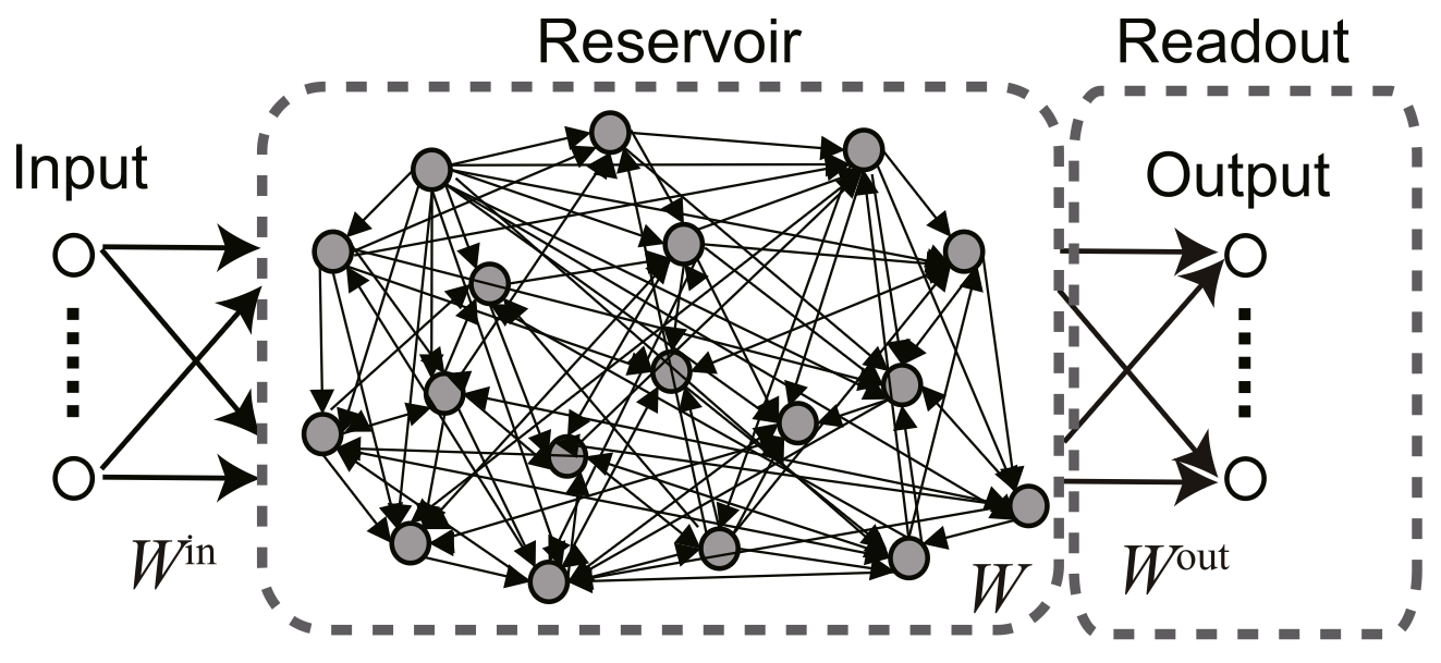
Figure 1: Reservoir computing system, with a dynamically evolving reservoir network that responds to inputs with complex activity states over time, and does not learn, and a readout output layer that is trained to extract the relevant states from the reservoir.

The reservoir network is typically initialized with random synaptic weights, and must have bidirectional connectivity (i.e., recurrence) which allows the activation state to reverberate over time, such that new input signals are automatically mixed in together with activity traces reflecting the prior inputs. This provides a temporally integrated, high-dimensional signal that naturally provides a useful basis space for extracting relevant spatiotemporal patterns of relevance, as determined by the target signals that train the output units.

Mathematically, successful reservoir network configurations are those that lie just at the edge of criticality, which exhibit more chaotic behavior (Langton, 1990). This can be assessed in terms of the Lyapunov exponent of the system, which is effectively the magnitude of the largest eigenvector of the network. This should be just below 1 to remain at the edge of criticality. An eigenvalue of greater than one means that the system will exhibit exponential growth in its activity over time, while a value much lower than 1 corresponds to a strongly damped system where activity dies out quickly.