
Error backpropagation
Error backpropagation (“backprop”) is a relatively straightforward mathematical procedure for performing error-driven learning, derived directly from the chain rule of basic calculus. It starts with an objective function that defines how to compute the error. To determine how to update synaptic weights to minimize this error, the first-order partial derivative of the objective function with respect to a given weight value can be computed using the chain rule, which thereby defines the error gradient. The synaptic weights are iteratively updated along the direction of this gradient. Many different techniques can be used to implement this error minimization procedure, including using higher-order derivatives.
The current generation of software tools used in abstract neural network models have the ability to automatically compute these error gradients directly from the chain of equations used in a model, which greatly simplifies the process of constructing complex novel models, and has been a major contributor to the explosive growth of research and progress in this field. For example, the widely used PyTorch framework has Autograd. Before the advent of such tools, people used to manually perform the relevant calculus and program in the resulting equations.
Consistent with its basis in fundamental principles of calculus and function optimization, backprop has been “invented” by a number of people over the years, including Widrow & Hoff (1960) and Werbos (1974). However, Rumelhart et al. (1986) were the last to invent it, which means they were the most successful in articulating and demonstrating the important properties of this learning procedure in the context of a comprehensive overall framework for modeling neurally inspired learning (Rumelhart & McClelland, 1986; McClelland & Rumelhart, 1986).
All of the widely used modern abstract neural network models today are based primarily on backprop, including large language models (LLMs), providing a clear demonstration of the computational power of this technique, and of error-driven learning more broadly. The surprising power of this procedure provides an important case where very high dimensional spaces can be efficiently searched using a dedicated-weight-gradient-search method, as discussed further in the context of search as a universal computational framework.
The literal mathematical procedure for computing backprop is inconsistent with the known properties of the brain, as famously pointed out by Crick (1989). However, the generec (generalized recirculation) approximation to backprop (O’Reilly, 1996; Lillicrap et al., 2020) provides a mechanism for powerful error-driven learning that is consistent with biological mechanisms, as elaborated in the even more biologically detailed kinase algorithm, which leverages the key principle of a temporal derivative for computing error gradients.
The most commonly used technique to perform gradient descent in backprop models, including in the original work of Rumelhart et al. (1986), is online, stochastic gradient descent. In this case, small, randomly chosen subsets of input patterns are used to compute the error gradients and update the synaptic weights (“online”) before proceeding to the next input patterns. This is contrasted with batch mode learning where the gradients are computed across all input patterns prior to updating the synaptic weights. Intuitively, the online form allows the network to more rapidly explore promising gradient directions and it breaks a lot of “ties” that otherwise occur when considering all of the input patterns at once: it is a more “decisive” form of learning, as contrasted with trying to simultaneously satisfy all of the constraints across all patterns, all at once.
Derivation of backprop
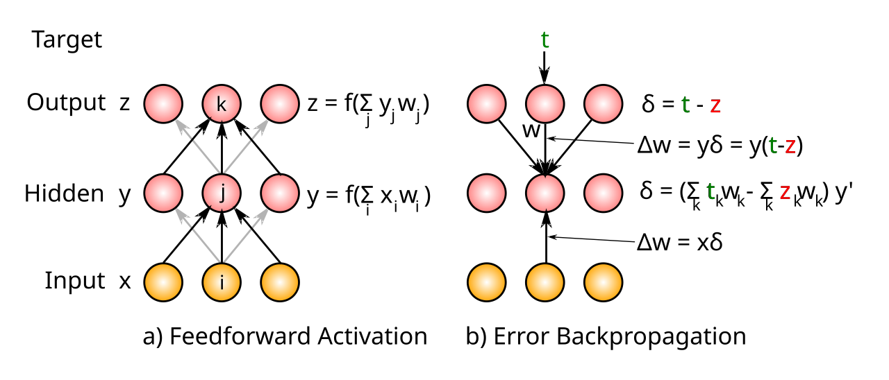
Figure 1: Illustration of backpropgation computation in three-layer network. First, the feedforward activation pass generates a pattern of activations across the units in the network, cascading from input, to hidden to output. Then, δ (delta) values are propagated backward in the reverse direction across the same weights. The delta sum is broken out in the hidden layer to facilitate comparison with the GeneRec algorithm, and the learning rate factor is omitted for simplicity.
Even though the software can compute the gradients for you automatically, it is important to work through the logic of the backpropagation calculus to actually understand what is going on, and especially to understand different ways of performing these computations in a more biologically plausible manner, as in the GeneRec algorithm. Figure 1 shows how it works in the case of a simple 3 layer feedforward network.
Feedforward activation
First, as shown in the left panel of Figure 1, we define the feedforward activation flow from Input to Hidden to Output:
\[ \eta_j = \sum x_i w_{ij} \]
\(\eta_j\) is the linear net input to hidden unit \(j\), computed as the dot product of sending activity \(x_i\) times the synaptic weight values (see linear algebra for an illustration, and Computing input conductances for biological context).
The unit activity (representing something like the expected rate of neural spiking in biological terms) is then a function of this net input:
\[ y_j = f(\eta_j) \]
The exact form of this function f is not critical, as long as it is differentiable (i.e., you can compute the derivative of it with respect to the linear net input factor). The standard function used in models from the 1980’s was the sigmoid (s-shaped) logistic function:
\[ f_l(x) = \frac{1}{1 + e^{-x}} = \frac{e^{-x}}{1 + e^{-x}} \]
This function has the biologically realistic property of a saturating nonlinearity, where increasingly large net inputs produce increasingly small additional increments in activation value, consistent with a maximum sustained firing rate of neurons in the neocortex of about 100 hz.
The derivative of this function has a nice simple form:
\[ f_l'(x) = f_l(x) (1 - f_l(x)) \]
However, a major problem with this logistic function from a practical perspective is that it causes an exponential decay of the error signal across layers in a multilayer (“deep”) neural network, which is one major reason that these early networks did not typically work well when adding more such hidden layers. This is known as the vanishing gradients problem. Also, the computation of the exponential function is relatively slow on a digital computer.
For these reasons, modern backpropagation networks typically use the ReLU rectified linear unit function, which is piecewise linear:
\[ f_r(x) = \rm{max}(0, x) \]
such that the activation is 0 for all net input levels below 0, and is otherwise purely linear. The derivative is likewise a piecewise function that is 0 or 1. See Key advances in ANNs in relation to neuroscience for more discussion.
Error function
Once the activity reaches the Output layer, it is compared with target values via an error function, such as the widely used Sum Squared Error (SSE):
\[ SSE = \sum_k \left( t_k - z_k \right)^2 \]
This is linear across neurons and thus easy to differentiate with respect to any given unit. Historically the cross-entropy (CE) error function was also used, because its derivative would cancel out the derivative of the logistic, making the math a bit simpler.
Error gradient chain rule
Now we finally get to the heart of the computation, which is to minimize the error (SSE) by changing the synaptic weights throughout the network. That is what error-driven learning means in this context. In particular, the biggest challenge from a calculus perspective is to figure out how to change the weights from the Input to the Hidden units, because this requires several steps of the chain rule:
\[ \Delta w_{ij} \propto -\frac{\partial SSE}{\partial w_{ij}} \]
This expression captures the idea that to know how to change the weights from input unit \(x_i\) to hidden unit \(y_j\), we have to know how changes in this weight \(w_{ij}\) are related to changes in the SSE, which is what the partial derivative expression tells us. The minus sign indicates that we want to minimize error, not maximize it, so we go in the opposite direction of this derivative.
By referring to Figure 1, you can see that the chain rule expansion of the basic activation function through hidden units \(j\) and output units \(k\) results in the following expansion of the above expression:
\[ -\frac{\partial SSE}{\partial w_{ij}} = -\frac{\partial SSE}{\partial z_k} \frac{\partial z_k}{\partial \eta_k} \frac{\partial \eta_k}{\partial y_j} \frac{\partial y_j}{\partial \eta_j} \frac{\partial \eta_j}{\partial w_{ij}} \]
Although this looks like a lot, each step is easily computed, and in practice it results in a simple recursive computation that cascades backwards across layers in much the same way that the feedforward activation sweep happens. In verbal terms, it involves computing how the SSE changes with output activity, how output activity changes with its net input, how this net input changes with hidden unit activity \(y_j\), how in turn this activity changes with its net input \(\eta_j\), and finally, how this net input changes with the weights from sending unit \(x_i\) to hidden unit \(y_j\).
Once all of these factors are computed, they can be multiplied together to determine how the weight \(w_{ij}\) should be adjusted to minimize error, and this can be done for all sending units to all hidden units, and with a shorter version of this chain, for all hidden units to all output units. The resulting expression is:
\[ -\frac{\partial SSE}{\partial w_{ij}} = \sum_k (t_k - z_k) * z_k' * w_{jk} * y_j' * x_i \rightarrow \]
Note that the negative of \(\partial SSE / \partial z_k\) is \(2 (t_k -z_k)\) and since 2 is a constant, we can just absorb it into the learning rate parameter.
To simplify things further, we can define an error gradient variable \(\delta\) for each unit, which represents the partial derivative of the error for that unit. In these terms, the \(\delta_j\) for a hidden unit in terms of the \(\delta_k\) for the output layer units is:
\[ \delta_j = \left( \sum_k \delta_k w_{jk} \right) y' \]
This form clearly shows the simpler recursive nature of the computation, which involves propagating the “delta” value backward across the weights, in the opposite direction that the activation typically flows in the “feedforward” direction. This is the essence of backpropagation. The need for different equations going in the feedforward vs. feedback direction contrasts with the temporal derivative mechanism used in Axon and the kinase algorithm.
The resulting learning rule in these terms is thus simply:
\[ \Delta w_{ij} = \epsilon \delta_j x_i \]
where \(\epsilon\) is a learning rate factor that controls the step size along the error gradient at each weight update.
Delta rule
If we focus on the synapses from the Hidden layer to the Output layer, or consider a simpler two-layer version of the network that just goes straight from Input to Output without a Hidden layer (i.e., a Perceptron; Rosenblatt, 1962; Minsky & Papert, 1969), the chain rule is shorter and you end up with an equation known as the delta rule, which is mathematically equivalent to the Rescorla-Wagner learning rule for reinforcement learning (Rescorla & Wagner, 1972; see also Widrow & Hoff, 1960 and Sutton & Barto, 1981).
Here is a simple form of the delta rule for an output unit with activation y receiving from an input unit with activation x, with weighted synapse value w:
\[ \Delta w = (t - y) x \]
where t is the target value.
Credit assignment
The delta rule and Eq 11 show that the essence of error-driven learning is a simple product of an error signal times the sending unit activation. This modulation of weight change by activity of the sending unit achieves a critical credit assignment function (or rather blame assignment in this case), so that when an error is made at the output, weights should only change for the sending units that contributed to that error. Sending units that were not active did not cause the error, and their weights are not adjusted.
Backpropagation to activations
The error gradient as computed in Eq 10 can also be used to directly update the activation state of units in the network, moving them in the direction that they should change once the weight changes are made:
\[ y^+ = y + \lambda \delta \]
where \(y^+\) represents a plus phase activation value by analogy with the equivalent computation performed by the GeneRec algorithm, and \(\lambda\) is a learning-rate-like factor that determines how much of the gradient to add.
Thus, this new activation value represents a more correct optimized representation of the current input state. In an Axon network with full bidirectional connectivity, the activation states are even more optimized by performing constraint satisfaction processing over multiple iterations, in addition to having a plus-phase activity state that specifically includes the error gradient as in Eq 13 (see GeneRec for the mathematical analysis).
In the standard feedforward backpropagation network, it is not clear what the use of the \(y^+\) activation state should be, however. This activation value is not what the other neurons in the network have seen: it would require an additional iteration to update all of the activations based on these updated values, which would mean that the error gradients themselves need to be updated, and so on. One solution to this question is given by the Almeida-Pineda version of recurrent backpropagation (Almeida, 1987; Pineda, 1988), which effectively iterates until the network activations stabilize. This is effectively what happens in the GeneRec model, as shown there.