
Temporal derivative
The temporal derivative is the change over time in the activity states of neurons, and it is the central mechanism for error-driven learning in Axon, via the kinase algorithm, building on the mathematical framework of GeneRec. In the predictive learning context, time can be discretized into two distinct phases (as originally developed in the Boltzmann machine):
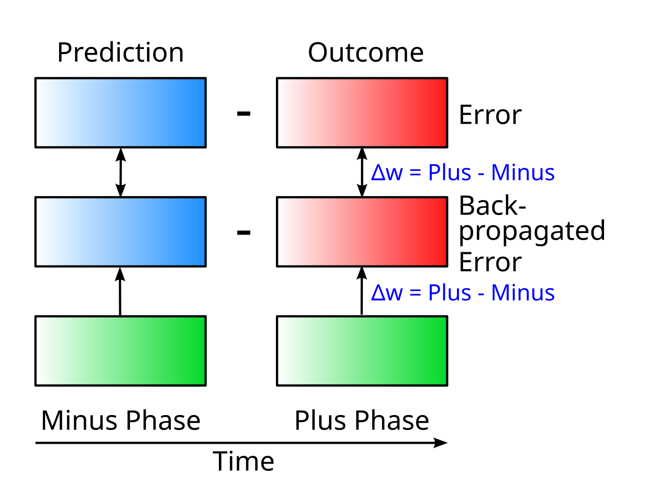
Figure 1: Temporal derivative learning is based on the change over time in neural activity states, e.g., as discretized into an initial Minus phase where the network is making a prediction, and a subsequent Plus phase where the actual outcome is experienced. Synapses everywhere can learn on this temporal difference, without requiring a separate structural pathway to convey the error, and error signals can arise from anywhere in a bidirectionally connected network, which are key advantages of using these differences over time.
- • The Minus phase is when the network is generating a prediction.
- • The Plus phase is when the network is experiencing the actual outcome (what actually happened).
The temporal derivative is the difference between these two phases, i.e., the prediction error, and every neuron in the network learns as a function of this difference:
- • Learning \(\propto\) (Plus - Minus)
In simple equation form, the change in synaptic weight \(w\) is a function of the phase-wise difference in activity state \(y\) between the plus phase (\(y^+\)) and minus phase (\(y^-\)):
\[ \Delta w \propto y^+ - y^- \]
By contrast, in standard error backpropagation learning, error signals are propagated via structurally separate pathways, using distinct equations from those governing activation propagation, which is the primary source of biological implausibility.
A key advantage of a temporal derivative is that time happens everywhere in a network, allowing an error signal to spread over time to all areas in the network of neurons in the brain. By contrast, derivatives computed between different anatomical pathways require these pathways to remain at least somewhat segregated and organized within the network, which typically would end up strongly constraining the kinds of error signals that can be computed.
Thus, a temporal derivative is a very robust, general-purpose mechanism of the sort that one might be particularly suited to the messy, organic world of biology. Indeed, initial empirical support for this mechanism is reported in Jang et al (2026) (see also OReilly (2026) Cortical Learning). Outside of the neocortex, the TD (temporal differences) algorithm for reinforcement learning shares the same temporal prediction error framework but maps onto very different neural substrates, in the form of dopamine.
Local computation of the temporal derivative
Another appealing property of the temporal derivative is that it can be computed locally at each neuron and synapse, through a competition between two chemical processes with different exponential integration time constants. Specifically, if you subtract a slower process from a faster one, then this automatically computes a temporal derivative.
This is illustrated in the following simple simulation, which shows the response to a “driver” input that drives the fast and slow chemical processes (using online exponential integration). In the brain, this driver is neural activity in the form of pre and post-synaptic spiking, which is integrated by a series of chemical pathways driven mainly by the influx of Calcium ions (see synaptic plasticity and the kinase algorithm for details).
The driver input changes over time in a manner consistent with predictive learning: there is an initial prediction value, and then a subsequent outcome value (Figure 1). The prediction is the local neural activity associated with the brain state present when generating a prediction of what will happen next, and the outcome is this local activity when experiencing the actual outcome, immediately after making the prediction.
The prediction error is represented by the difference between the fast and slow traces at the end of the time window when the sequence of prediction-then-outcome has completed. If this difference is positive, that reflects a positive-valued error gradient, and synaptic weights should correspondingly increase (known as LTP in the synaptic plasticity literature). Likewise, if it is negative, the synaptic weights should decrease (LTD).
Temporal Derivative from Fast - Slow
fastTau := 20.0 // time constant for fast integration
slowTau := 40.0 // time constant for slow integration
pred := 50.0
out := 80.0
var dwtStr, fastStr, slowStr, predStr, outStr string

##
totalTime := 200
driver := zeros(totalTime) // driver is what is driving the system
fast := zeros(totalTime) // fast is a fast integrator of driver
slow := zeros(totalTime) // slow is a slow integrator of driver
##

func td() {
    fastStr = fmt.Sprintf("Fast Tau: %g", fastTau)
    slowStr = fmt.Sprintf("Slow Tau: %g", slowTau)
    predStr = fmt.Sprintf("Prediction: %g", pred)
    outStr = fmt.Sprintf("Outcome: %g", out)
    ##
    d := array(pred) // current drive
    f := 0.0 // current fast
    s := 0.0 // current slow
    fTau := array(fastTau)
    sTau := array(slowTau)
    ##
    for t := range 200 {
        if t == 150 {
            # d = array(out)
        }
        ##
        f += (1.0 / fTau) * (d - f) // f moves toward d
        s += (1.0 / sTau) * (d - s) // s moves toward f
        driver[t] = d
        fast[t] = f
        slow[t] = s
        ##
    }
    ##
    dwt := fast[-1] - slow[-1]
    ##
    dwtStr = fmt.Sprintf("<b>Weight Change ΔW ≅ Predition - Outcome = Fast - Slow = %7.2g</b>", dwt.Float1D(0))
}

td()

plotStyler := func(s *plot.Style) {
    s.Range.SetMax(100).SetMin(0)
    s.Plot.XAxis.Label = "Time"
    s.Plot.XAxis.Range.SetMax(200).SetMin(0)
	s.Plot.Legend.Position.Left = true
}
plot.SetStyler(driver, plotStyler)

fig1, pw := lab.NewPlotWidget(b)
dl := plots.NewLine(fig1, driver)
fl := plots.NewLine(fig1, fast)
sl := plots.NewLine(fig1, slow)
fig1.Legend.Add("Driver", dl)
fig1.Legend.Add("Fast", fl)
fig1.Legend.Add("Slow", sl)


dwtTx := core.NewText(b)
dwtTx.Styler(func(s *styles.Style) {
    s.Min.X.Ch(80) // clean rendering with variable width content
})
core.Bind(&dwtStr, dwtTx)

func updt() {
    td()
    dl.SetData(driver)
    fl.SetData(fast)
    sl.SetData(slow)
    dwtTx.UpdateRender()
    pw.NeedsRender()
}

func addSlider(label *string, val *float64, mxVal float32) {
    tx := core.NewText(b)
    tx.Styler(func(s *styles.Style) {
        s.Min.X.Ch(40)  // clean rendering with variable width content
    })
	core.Bind(label, tx)
	sld := core.NewSlider(b).SetMin(1).SetMax(mxVal).SetStep(1).SetEnforceStep(true)
	sld.SendChangeOnInput()
	sld.OnChange(func(e events.Event) {
		updt()
		tx.UpdateRender()
	})
	core.Bind(val, sld)
}

addSlider(&predStr, &pred, 100)
addSlider(&outStr, &out, 100)
addSlider(&fastStr, &fastTau, 100)
addSlider(&slowStr, &slowTau, 100)
The code for this simulation updates the fast and slow variables according to a simple running-average update equation, e.g., for the \(fast\) variable:
\[ \rm{fast} += \frac{1}{\rm{fastTau}} (\rm{driver} - \rm{fast}) \]
This equation causes the variable (fast or slow) to move toward the driver value at a rate determined by the “tau” time constant factor. For example, if the driver is larger than fast, then \(driver - fast\) is positive, so fast will increase to approach the value of the driver. If \(fastTau = 10\), then it moves a 10th of the way toward the driver at each update (and gets roughly 2⁄3 of the way to the driver in fastTau steps). This very simple type of update equation is used throughout axon and is likewise very prevalent in biology.
Some things you can try:
• Increase or decrease both Prediction and Outcome by the same amount: observe that the weight change is only sensitive to the relative differences, due to the competitive, subtraction logic between Fast - Slow.
• Set both Prediction and Outcome to the same value (e.g., 50), and observe that this results in zero weight change, which is consistent with there being no error in the prediction relative to the outcome. This holds even when you significantly increase or decrease the raw values, e.g., both 20 or both 80. This is a critical point of contrast with hebbian forms of learning, which are typically driven by the overall levels of activity, such that you would expect (larger) weight increases with more activity.
• There are important constraints on the Tau factors too. For example, with Prediction and Outcome both at 50, increase Slow Tau up to 70. You can see that the weight change is positive now, even though there is no prediction error, just because the Slow factor is too slow to catch up at the end. This means that the local chemical rate constants that produce these Tau factors must be properly tuned for the actual temporal dynamics of the network-level error signals.
Although this might be considered biologically implausible, in fact there is strong evidence of prominent oscillatory rhythms in the brain at different characteristic frequencies, including the alpha cycle at roughly 10 Hz (100 ms period) and the theta cycle at roughly 5 Hz (200 ms period). These rhythms have been shown to strongly influence learning, in a manner consistent with this simple model and the kinase algorithm more generally.
In summary, Sim 1 based on the competition between two simple exponential integration equations (Eq 2) demonstrates that a locally computed temporal derivative can drive synaptic changes in a manner consistent with an error signal that emerges over time.
Timing of learning
A critical issue with this temporal derivative framework is that the accurate computation of a prediction error signal must happen at some point after the onset of the actual outcome. If learning happened during the minus (prediction) phase for example, it would learn toward the prediction state and away from the prior outcome state!
Furthermore, the timing must allow the fast component sufficient time to deviate from the slow component, but not too much time, because then the difference will start to go away as the slow component catches up. In many Axon simulations, the inputs are presented at regular intervals for the sake of simplicity, and learning timing can be driven algorithmically. But how could it actually work in the brain?
There is a reliable timing signal available at each individual neuron, which could potentially drive the biological synaptic plasticity process, as illustrated in the following simulation. This signal is based on the way that the absolute value of the difference between fast – slow evolves over time, plotted as diff:
Timing for learning
fastTau := 20.0 // time constant for fast integration
slowTau := 40.0 // time constant for slow integration
pred := 50.0
out := 80.0
var dwtStr, fastStr, slowStr, predStr, outStr string

##
totalTime := 200
driver := zeros(totalTime) // driver is what is driving the system
fast := zeros(totalTime) // fast is a fast integrator of driver
slow := zeros(totalTime) // slow is a slow integrator of driver
diff := zeros(totalTime) // diff is the absolute value of fast - slow diff
##

func td() {
    fastStr = fmt.Sprintf("Fast Tau: %g", fastTau)
    slowStr = fmt.Sprintf("Slow Tau: %g", slowTau)
    predStr = fmt.Sprintf("Prediction: %g", pred)
    outStr = fmt.Sprintf("Outcome: %g", out)
    ##
    d := array(pred) // current drive
    f := 0.0 // current fast
    s := 0.0 // current slow
    fTau := array(fastTau)
    sTau := array(slowTau)
    ##
    for t := range 200 {
        if t == 150 {
            # d = array(out)
        }
        ##
        f += (1.0 / fTau) * (d - f) // f moves toward d
        s += (1.0 / sTau) * (d - s) // s moves toward f
        driver[t] = d
        fast[t] = f
        slow[t] = s
        diff[t] = abs(s-f)
        ##
    }
    ##
    dwt := fast[-1] - slow[-1]
    ##
    dwtStr = fmt.Sprintf("<b>Weight Change ΔW ≅ Predition - Outcome = Fast - Slow = %7.2g</b>", dwt.Float1D(0))
}

td()

plotStyler := func(s *plot.Style) {
    s.Range.SetMax(100).SetMin(0)
    s.Plot.XAxis.Label = "Time"
    s.Plot.XAxis.Range.SetMax(200).SetMin(0)
	s.Plot.Legend.Position.Left = true
}
plot.SetStyler(driver, plotStyler)

fig1, pw := lab.NewPlotWidget(b)
dl := plots.NewLine(fig1, driver)
fl := plots.NewLine(fig1, fast)
sl := plots.NewLine(fig1, slow)
dfl := plots.NewLine(fig1, diff)
fig1.Legend.Add("Driver", dl)
fig1.Legend.Add("Fast", fl)
fig1.Legend.Add("Slow", sl)
fig1.Legend.Add("Diff", dfl)


dwtTx := core.NewText(b)
dwtTx.Styler(func(s *styles.Style) {
    s.Min.X.Ch(80) // clean rendering with variable width content
})
core.Bind(&dwtStr, dwtTx)

func updt() {
    td()
    dl.SetData(driver)
    fl.SetData(fast)
    sl.SetData(slow)
    dfl.SetData(diff)
    dwtTx.UpdateRender()
    pw.NeedsRender()
}

func addSlider(label *string, val *float64, mxVal float32) {
    tx := core.NewText(b)
    tx.Styler(func(s *styles.Style) {
        s.Min.X.Ch(40)  // clean rendering with variable width content
    })
	core.Bind(label, tx)
	sld := core.NewSlider(b).SetMin(1).SetMax(mxVal).SetStep(1).SetEnforceStep(true)
	sld.SendChangeOnInput()
	sld.OnChange(func(e events.Event) {
		updt()
		tx.UpdateRender()
	})
	core.Bind(val, sld)
}

addSlider(&predStr, &pred, 100)
addSlider(&outStr, &out, 100)
addSlider(&fastStr, &fastTau, 100)
addSlider(&slowStr, &slowTau, 100)
You can see that across different combinations of prediction and outcome driver states, the diff value exhibits two distinct peaks: one at the start when the onset of prediction-phase activity drives fast and slow to change at their different rates, and another just after onset of the outcome (plus) phase. The first peak is generally much larger and more reliable in practice, reflecting changes in the overall sensory or internal (hidden) state of the network, while the second peak is proportional to the difference in the prediction versus outcome.
In primates for example, there is robust evidence for characteristic waves of neural activity following saccades, known as event-related potentials (ERPs) (Helfrich & Knight, 2019), with the modal saccade fixation tightly centered at around 200 ms (Devillez et al., 2020). Furthermore, higher-order thalamus areas that interconnect with the neocortex (i.e., pulvinar and mediodorsal) drive strong theta-rhythm (5 Hz, 200 ms) intrinsic oscillations that have significant impacts on attention and behavior (Fiebelkorn & Kastner, 2019; Fiebelkorn & Kastner, 2021).
In rodents, there is evidence of brain-wide entrainment of neural activity at the theta cycle (also with a 200 ms period) (Sattler & Wehr, 2025), with strong evidence of overall cortex-wide neural activity characterized by periods of relative stability with rapid transitions between (i.e., meta-stability; La Camera et al., 2019; Recanatesi et al., 2022). These phasic transitions appear to be driven in part by motor events, consistent with the broad cortex-wide connectivity of the VA (ventral anterior) thalamus, receiving motor and prefrontal cortex inputs (see frontal thalamus).
In our models, we have found that driving the timing of learning to occur a fixed number of cycles (milliseconds) after the onset of the first peak works well in practice. In a spiking network (e.g., the kinase algorithm for Axon), the time integrated values that drive learning are not nearly as smooth as those in Sim 2, because they have a significant contribution from postsynaptic spiking. However, much smoother values are available in the total excitatory and inhibitory conductances coming into each neuron, which sample from a large number of other neurons. The same peak-driven logic works well in this case, and is used in the kinase algorithm.