
Kinase algorithm
The kinase learning algorithm is an abstraction of the detailed chemical pathways involved in synaptic plasticity, which are mediated by kinases including CaMKII and DAPK1 that play central roles in these learning processes. This algorithm accomplishes error-driven learning via a temporal derivative computed between the faster CaMKII-mediated pathway and the slower DAPK1-mediated pathway, which are known to be in competition with each other (Goodell et al., 2017; Goodell et al., 2021; Cook et al., 2021; Tullis & Bayer, 2023; Bayer & Giese, 2025).
The relevant background for this algorithm is presented in the following pages:
• Synaptic plasticity reviews the relevant neuroscience for how synapses change their effective strength (weight), and the critical contributions of kinases to this process.
• Temporal derivative provides a high-level account for the essential computational principles behind this algorithm, including an interactive simulation of how a competitive interaction between fast and slow pathways can compute the error gradient at the heart of error-driven learning.
• GeneRec derives a concrete learning algorithm directly from the mathematics of error backpropagation, which uses bidirectional connectivity to propagate error gradients throughout the neocortex. The kinase algorithm leverages the same principles at a computational level, while using more directly biologically based mechanisms that also have some important quantitative differences in the gradients computed.
• Jang et al (2026) presents initial direct evidence showing that the direction of synaptic plasticity in neurons recorded in the mouse CA1 area is consistent with the temporal derivative hypothesis.
• OReilly (2026) Cortical Learning provides a concise summary motivating the approach across different levels of analysis.
Here, we build on these foundations to describe the detailed mechanisms that actually drive learning in the Axon models, which represent an attempt to satisfy constraints from neuroscience, computational efficacy, and computational cost.
At a big-picture level, the two central ideas behind the kinase algorithm are:
• Use biophysically grounded equations for computing the synaptic Ca++ influx via the NMDA and VGCC channels that are well-established as the primary initial drivers of synaptic plasticity. NMDA is sensitive to the conjunction of pre and postsynaptic activity, while VGCCs (voltage-gated calcium channels) are driven in a sharply phasic manner by backpropagating action potentials from the receiving neuron.
• Apply a cascade of simple exponential integration steps to simulate the complex biochemical processes that follow from this Ca++ influx, with time constants optimized based on computational performance across a wide range of tasks. The final two steps in this cascade implement the temporal derivative computation where the faster penultimate step drives LTP (weight increases) while the final slower step drives LTD (weight decreases).
This strategy leverages biophysically constrained mechanisms where they are well-established, while adopting a more abstracted computationally motivated approach to the complexities of the subsequent biochemical processes, which are not yet sufficiently specified to support a more bottom-up approach. The overall mechanism behind the temporal derivative is supported by the general properties of the CaMKII and DAPK1 kinases and related mechanisms, as described in synaptic plasticity, and by the initial empirical results of Jang et al (2026).
However, at a pragmatic implementational level, it would be very expensive to compute the Ca++ influx based on the NMDA and VGCC biophysical equations for each synapse individually, given that synapses greatly outnumber neurons (e.g., \(N^2\) in a fully connected model), Therefore, we instead break out the computation into two subcomponents:
• A shared dendrite-level Ca++ value that reflects the overall dendritic membrane potential and the contributions of backpropagating action potentials from the receiving neuron on the NMDA and VGCC channels.
• An efficiently computed synapse-specific multiplier, that reflects the specific coincident pre and postsynaptic activity at each synapse.
In another example of the synergies between neuroscience and computation, these two terms can be directly associated with the two essential terms in the error backpropagation learning rule, which are the error gradient and the credit assignment factors:
\[ \Delta w \propto \rm{Error} * \rm{Credit} \]
These are concretely expressed in terms of \(\delta\) and the sending unit activity \(x\) in error backpropagation:
\[ \Delta w \propto \delta x \]
In the kinase algorithm, the Error factor is computed from the dendrite-level Ca++, and the synapse-specific multiplier provides the Credit assignment. The computational-level properties of these two factors are overall consistent with the backpropagation versions, but also have important differences that are beneficial for the discrete spiking nature of the Axon framework, and also help reduce the vanishing gradient problem in deep networks. Thus, although this separation into these two distinct factors is motivated by computational cost considerations, it nevertheless provides a useful basis for understanding the functional properties of the putative biologically based learning mechanism driven by NMDA and VGCC Ca++ influx.
Due to the continuous-time nature of the Axon model, which simulates neural dynamics at the 1 ms per cycle timescale, it takes roughly 200 cycles for each “trial” of processing to unfold, corresponding to a theta rhythm. The kinase algorithm provides an account of how information accumulates to drive effective learning based on the statistics of pre and postsynaptic spiking over this 200 ms window.
In the predictive learning framework typically used, this time window encompasses an iteration of prediction (minus phase) followed by an outcome (plus phase), and then learning occurs at the end of the plus phase. The specific events that could trigger this learning in a biologically realistic manner are described below. Aside from this temporal discretization of the learning process (and external dynamics of the environment), all of the other equations in Axon operate continuously over time, providing a real-time model of actual neural processing.
There are also longer timescale synaptic processes included in the kinase algorithm, which significantly improve the stability of learning over time, detailed below (Stabilization and rescaling mechanisms). These processes are motivated by a range of neuroscience mechanisms, including those operating during sleep.
Error gradient via dendritic Ca++
The overall Ca++ influx across all the dendrites of a simulated neuron is computed using the biophysically based NMDA conductance model described in neuron channels, and a simple spike-driven approximation to the VGCC conductance. The NMDA contribution starts with the conductance:
\[ g_{nmda}(t) = \frac{g_{e-raw}(t) \overline{g}_{nmda}}{1 + \frac{[Mg^{++}]}{3.57} e^{-0.062 V_d}} - \frac{1}{\tau_d} g_{nmda}(t-1) \]
where \(V_d\) is the dendritic membrane potential (see neuron dendrites) and the \(g_{e-raw}(t)\) factor is the raw excitatory synaptic input described in Computing input conductances, reflecting the total potential glutamate released from presynaptic neurons that could bind to and open NMDA receptors, which is mathematically equivalent to the net input in abstract neural network models:
\[ g_{e-raw}(t) = \frac{1}{n} \sum_i x_i w_i \]
The NMDA conductance drives a Ca++ influx level using the following equation from the Urakubo et al. (2008) model (see model details and Sabatini et al., 2002):
\[ \rm{Ca}_{nmda}(t) = \frac{- g_{nmda}(t) V_d}{1 - e^{0.0756 V_d}} \]
The VGCC Ca++ influx occurs in a highly circumscribed time window around the spiking of the receiving neuron, and can be efficiently computed using a simple spike-driven impulse function with a decay factor (\(\tau_d = 10 ms\)):
\[ \rm{Ca}_{vgcc}(t) = \rm{Spike} * 35 - \frac{1}{\tau_d} \rm{Ca}_{vgcc}(t-1) \]
The total resulting dendritic Ca++ influx is just the sum of these two terms, with a normalization factor (80) that results in approximately normalized values that work well in practice in the learning rule:
\[ \rm{Ca}_{tot}(t) = \frac{1}{80} \left( \rm{Ca}_{nmda}(t) + \rm{Ca}_{vgcc}(t) \right) \]
Kinase cascade
As described in more detail in synaptic plasticity, the influx of Ca++ ions via NMDA and VGCC channels then drives a complex cascade of chemical reactions involving various kinases and phosphatases, along with other molecules and critical binding dynamics, to ultimately drive changes in excitatory AMPA receptor number and efficacy, which is the end result of learning (see the Urakubo08 simulation for a detailed model of some of these processes).
Table 1: Kinase time constants
| Parameter | Value |
|---|---|
| CaM \(\tau_{cam}\) | 2 ms |
| CaP \(\tau_{cap}\) | 40 ms |
| CaD \(\tau_{cad}\) | 40 ms |
| Syn \(\tau_{syn}\) | 30 ms |
Because it is computationally intractable to simulate these processes in biophysical detail at scale (and there is still a lot of uncertainty about how these things actually work), we use a simple approximation involving a cascade of exponential integration steps (time constants shown in Table 1), starting with the activation of calcium calmodulin (CaM) by the raw Ca++ influx:
\[ \rm{CaM}(t) = \frac{1}{\tau_{cam}} \left( \rm{Ca}_{tot}(t) - \rm{CaM}(t) \right) \]
This then drives the potentiation factor, which reflects the extent to which the CaMKII kinase is bound to the GluN2B binding site on the NMDA receptor that then drives LTP (synaptic weight increases), according to the structural model (Bayer & Giese, 2025):
\[ \rm{CaP}(t) = \frac{1}{\tau_{cap}} \left( \rm{CaM}(t) - \rm{CaP}(t) \right) \]
The final, slowest step in the cascade is the depression factor that reflects the activation of the DAPK1 kinase and binding at the Thr305/306 site on the CaMKII kinase, which drive LTD (synaptic weight decreases):
\[ \rm{CaD}(t) = \frac{1}{\tau_{cad}} \left( \rm{CaP}(t) - \rm{CaD}(t) \right) \]
In the temporal derivative framework, CaP is the faster, potentiation process while CaD is the slower, depression process, and the subtraction of the two provides an approximation to the backpropagation error gradient:
\[ \delta \approx \rm{CaP} - \rm{CaD} \]
The kinase learning rule directly uses this delta factor, along with the Syn synaptic activity credit assignment factor described below:
\[ \Delta w \propto (\rm{CaP} - \rm{CaD}) \rm{Syn} \]
As noted above, this learning rule is applied after 200 ms of iterative updating of all of the above variables, which are plotted in Figure 1 across two 200 ms trials to provide a sense of their overall dynamics.
Note that because we are only using the difference between these factors, they are relatively robust to various missing components that would provide a constant offset contribution, such as a more detailed accounting of the Ca++ buffering dynamics. Also, while the direct cascading of CaD on top of CaP captures some of the temporal dynamics of CaMKII activation at Thr286 (which promotes potentiation) versus Thr305/306 (which promotes depression; Cook et al., 2021), there are also independent pathways modulating DAPK1 activity, but they are more indirect than the direct binding of CaM to activate CaMKII, and thus likely to be slower overall, which is the critical functional property.
Historically, the above cascaded exponential integration equations were originally developed for the Leabra XCAL learning rule (temporally eXtended Continuous Attractor Learning; O’Reilly et al., 2012), with some inspiration from biophysical cascades, but without as clear of an understanding of their direct mapping onto the CaMKII and DAPK1 kinase substrates.
Computational properties of the kinase error gradient
The kinase error gradient (Eq 11) has some important similarities and differences from the corresponding error backpropagation gradient, which can best be seen by comparison with the GeneRec approximation of this gradient:
\[ \delta \approx y^+ - y^- \]
This simple difference in two rate-code activation states is used to approximate the corresponding difference in linear net input factors times the derivative of the activation function:
\[ \delta = \left( \sum_i x_i^+ w_i - \sum_i x_i^- w_i \right) y' \approx y^+ - y^- \]
This is overall similar to the kinase error gradient, where the Ca++ influx is driven largely by the net input-like \(g_{e-raw}(t)\) term in Eq 4, but it is also modulated by both the dendritic membrane potential \(V_d\) (in both Eq 3 and Eq 5) and has a direct spiking-based contribution from VGCC (Eq 6). The subtraction of CaP – CaD in Eq 11 implicitly computes the derivative of these activation-based terms (\(V_d\) and spiking), as explained in the GeneRec derivation.
A key difference however is that these kinase activation-based values are overall much more graded than the traditional sigmoidal logistic activation function used in simple GeneRec models, and the related X-over-X+1 function used in the Leabra framework. Therefore, the end result is something closer to the behavior of error backpropagation using the linear ReLU activation function, where the activation derivative \(y'\) is just 1 for any active unit, such that the effective error gradient is effectively linear in the net inputs.
With a softer, more graded contribution of the activation factors in the kinase error gradient, they are also more linear in the underlying net input factors. The major consequence is that this error gradient should therefore more linearly reflect the error gradients across layers in deep networks with many such layers, thereby avoiding the vanishing gradient problem that plagued earlier backprop networks that used sigmoidal-like functions with saturating nonlinearity (see error backpropagation for details).
The fact that these activation factors nevertheless do retain a graded representation of the receiving neuron’s activity represents an important deviation from error backpropagation with ReLU activations, which only have a strictly binary contribution of receiving activity. If the receiving unit’s net input is less than 0, then it learns nothing at all about the current trial, and, somewhat counter-intuitively, if it is greater than 0, then there is actually no contribution of the receiving unit’s activity to the the magnitude of learning (all \(y'\) are 1 in Eq 14). This was not true when saturating nonlinearities were used. This behavior is inconsistent with the basic mechanisms of synaptic plasticity. Note that it is still true that the magnitude of the weights going up to the next layer influence the sign and magnitude of the error gradients, but these do not contribute to the activity of the hidden unit in a feedforward backpropagation network.
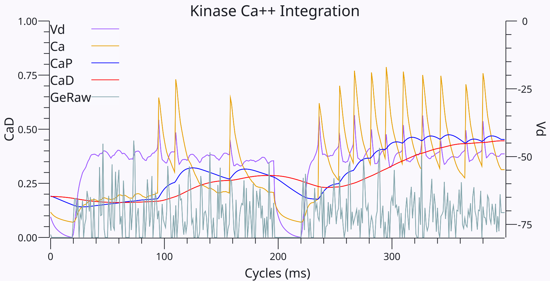
Figure 1: Example traces of Ca++ values across two different trials of 200 cycles (ms) each, showing the graded nature of the activation-based terms, which results in less of a vanishing gradient in kinase-based learning. The constant noisy background of presynaptic excitatory inputs (GeRaw; which is being offset by correspondingly high levels of pooled inhibition, not shown) results in a low-level elevation of the dendritic membrane potential (Vd) and thus a low level of total Ca++ (Ca). When the receiving neuron fires spikes, the NMDA and VGCC contributions to Ca increase dramatically, causing the cascaded integration of CaP and CaD to increase over time. However, in both of these trials, the final levels of CaP and CaD are roughly equal, so the error gradient is near zero and synaptic weights will not change.
The graded nature of these integrated Ca++ signals is shown in Figure 1, which plots the relevant variables over two different trials of 200 ms each.
Synaptic activity credit assignment
The second component of the kinase algorithm is the credit assignment factor, which captures the extent of coincident pre-post synaptic activity over time, which the NMDA receptor is strongly sensitive to. If we did not have real-world computational cost constraints, the aggregate NMDA Ca++ value computed in Eq 5 would instead be computed at each individual synapse, using local values, and this sensitivity would be directly manifest in the local synaptic Ca++ signal.
Instead, we use the following separate Syn synapse-specific factor to multiply the aggregate error-gradient term as shown in Eq 12. This activity factor starts with a spike-triggered decaying activity trace that is computed for each neuron, which reflects the net decay / buffering of intracellular Ca++ over time after a spike at the synaptic level, and is labeled CaSyn in the simulator:
\[ \rm{CaSyn}(t) = \frac{1}{\tau_{syn}} (\rm{Spike}(t) - \rm{CaSyn}(t-1)) \]
At each synapse, the sending * receiving neuron product of these traces is accumulated, using the same cascade of exponential integration factors (Eq 8 – Eq 10) driven by this product:
\[ \rm{SR}(t) = \rm{CaSyn}_s(t) * \rm{CaSyn}_r(t) \]
The longest time-integral of this SR value from the kinase cascade is then used as the Syn credit assignment value in Eq 12 (in theory CaP would be multiplied by the CaP-timescale integral, and CaD would be multiplied by the CaD timescale, but we just have one value and use the longer timescale as it defines the full span of the relevant values; also multiplying each dendritic factor by the corresponding Syn time integral did not work as well in larger networks).
Extensive empirical tests of the above credit assignment mechanism showed that it works significantly better in practice across a range of challenging tasks, relative to a range of other different possibilities that were explored. In particular, the fine-grained sensitivity of this mechanism to the coincidence of pre-and-post firing on the timescale of about 30 ms appears to provide a critical credit assignment factor for determining the extent to which different synapses should be modified in order to reduce the error gradients represented by the \(\delta\) factor.
At a computational level, the fact that this credit assignment factor is the product of both sending and receiving terms, and is sensitive to their temporal coincidence, represents a significant departure from the use of the sending activity only in error backpropagation. This difference should make the kinase algorithm more sensitive to correlated neural activity, and may play a role similar to Hebbian learning as a regularizer as used in the Leabra model.
Neuron-level linear approximation version
The synapse-specific SR(t) value in eq_trace-syn and its exponential integrations, though very simple, are still very computationally expensive to compute because the number of synapses is much greater than the number of neurons. Therefore, in practice we compute these values using a set of linear regression coefficients based on a vector of binned CaSyn values at the neuron level, with each bin holding the average CaSyn value over a period of 10 ms, which provides sufficient resolution to compute the necessary pre-post firing correlations.
At the point of learning, which occurs once at the end of a theta cycle of 200 ms typically, the values in each bin are multiplied for the sender * receiver at each synapse, and then the linear regression coefficients over these bin products are applied to directly compute the effective CaP and CaD time integral value that would otherwise be computed according to the above equations. These coefficients were trained using a combination of ridge and lasso regression based on 100 random Poisson spike trains per condition of a full combinatorial (outer product) sweep of minus and plus phase firing rates sampled in 10 hz increments from 0 – 120 hz for the pre and post neuron (12 * 12 * 12 * 12 = 20,736 frequency combinations * 100 trials = 2,073,600 total trials). The resulting coefficients have \(r^2\) values of 0.991 and 0.996 for CaP and CaD respectively (i.e,. they account for that proportion of the variance in the data). Thus, this method provides a highly accurate and significantly more performant way of computing these values at the synaptic level. See kinase/linear for details.
How does the synapse know when to learn?
What kind of biological signal causes learning to take place after the plus phase of activity, as opposed to a reversed sequence of an outcome phase followed by a subsequent prediction phase for example? Is there some distinctive neural signature that marks these phases so that the proper alignment occurs with sufficient reliability to drive effective learning?
There is always the possibility that a global neuromodulator signal could provide the critical “learn now” signal, and indeed norepinipherine has appropriate properties and projects widely into the neocortex. However, given the different timing of activity in different cortical areas, and the relatively localized nature of sensory prediction errors for example, it would be more robust for a local, neuron-level signal to guide the timing of learning.
As discussed in Timing of learning, there are two peaks of relative activity associated with the onset of the minus and plus phases, so that the minus phase peak can initiate the learning process, and the plus phase peak can finalize it. The total excitatory and inhibitory conductance impinging on a neuron, integrated over time, robustly and relatively smoothly exhibits these peaks in terms of the difference between a fast vs. slow integration of this activity, so we use that to drive learning timing.
The initial minus-phase peak is generally larger and more robust, so it dominates by triggering the start of the learning process. After a parameter-dependent number of cycles (milliseconds) from the onset of the minus-phase peak, the plus-phase peak is detected, and a specified number of cycles after that, the postsynaptic learning signal is recorded into the LearnDiff variable, to drive learning.
The peak-finding logic works robustly by recording the time and peak value whenever it exceeds the prior peak. This ratcheting-up dynamic continues until the empirical peak value is reached. When the time since the last peak exceeds the minimum minus cycle threshold, the peak baseline is reset and peak detection switches to finding the plus phase peak, using the same logic. When the cycles since that peak exceed the plus phase cycle parameter, learning occurs.
Although such mechanisms have not been specifically demonstrated in neurons, these are very “biologically friendly” mechanisms involving chemical integration over time, which is the basis for the biophysically detailed Urakubo et al. (2008) model for example. Furthermore, it is likely that various simpler single-peak and / or timing-driven dynamics could produce comparable results. When experimenting with various versions of the double-peak dynamics and earlier ideas, learning was generally robust as long as things didn’t get too far off from the plus phase.
Stabilization and rescaling mechanisms
A collection of biologically motivated mechanisms are used to provide a stronger “backbone” or “spine” for the otherwise somewhat “squishy” learning that emerges from the above error-driven learning mechanisms, serving to stabilize learning over longer time scales, and prevent parasitic positive feedback loops that otherwise plague these bidirectionally connected networks. These positive feedback loops emerge because the networks tend to settle into stable attractor states due to the bidirectional, generally symmetric connectivity, and there is a tendency for a few such states to get broader and broader, capturing more and more of the “representational space”.
The credit assignment process, which is based on activation, contributes to this “rich get richer” dynamic where the most active neurons experience the greatest weight changes. We colloquially refer to this as the “hog unit” problem, where a small number of units start to hog the representational space, and it represents a major practical barrier to effective learning if not managed properly. Metaphorically, it akin to corruption and extreme wealth inequality in the political or economic world: it reduces the overall efficiency of the system and can lead to significant breakdowns if it gets too severe.
Note that this problem does not arise in the vast majority of purely feedforward networks used in the broader neural network field, which do not exhibit attractor dynamics. However, this kind of phenomenon is problematic in other frameworks with the potential for such positive feedback loops, such as on-policy reinforcement learning, generative adversarial networks, or other forms of recurrent backpropagation networks such as backprop-through-time (BPTT; Lillicrap & Santoro, 2019; Linsley et al., 2020).
Continuing the above metaphor, various forms of equalizing taxation and wealth redistribution are required to level the playing field in these models. The set of stabilizing, anti-hog mechanisms in Axon include:
• SWt: structural, slowly adapting weights. In addition to the usual learning weights driven by the above equations, we introduce a slowly adapting, multiplicative weight value that represents the biophysical properties of the dendritic spine – the SWts “literally” give the model a spine!
As reviewed in synaptic plasticity spines are structural complexes where all the synaptic machinery is organized, and they slowly grow and shrink via genetically controlled, activity-dependent protein remodeling processes, primarily involving the actin fibers also found in muscles. A significant amount of spine remodeling takes place during sleep, so the SWt updating represents a simple model of sleep effects.
The SWt is multiplicative in the sense that larger vs. smaller spines provide more or less room for the AMPA receptors that constitute the adaptive weight value. The net effect is that the more rapid trial-by-trial weight changes are constrained by this more slowly adapting multiplicative factor, preventing more extreme changes. Furthermore, the SWt values are constrained by a zero-sum dynamic relative to the set of receiving connections into a given neuron, preventing the neuron from increasing all of its weights higher and hogging the space. The SWt is also initialized with all of the randomness associated with the initial weights, and preserving this source of random variation, preventing weights from becoming too self-similar.
• Homeostatic activity levels: There is extensive evidence from Gina Turrigiano and collaborators, among others, that synapses are homeostatically rescaled to maintain target levels of overall activity, which vary across individual neurons TorradoPachecoBottorffGaoEtAl21]. We simulate this process at the same slower timescale as updating the SWts (likewise associated with sleep), which are also involved in the rescaling process. The target activity levels can also slowly adapt over time, similar to an adaptive bias weight that absorbs the “DC” component of the learning signal ([[@Schraudolph98]], but this adaptation is typically subject to a zero-sum constraint, so any increase in activity in one neuron must be compensated for by reductions elsewhere.
This is similar to a major function performed by the BCM learning algorithm in the Leabra framework – by moving this mechanism into a longer time-scale outer-loop mechanism (consistent with Turigiano’s data), it works significantly more effectively. By contrast, the BCM learning ended up interfering with the error-driven learning signal, and required relatively quick time-constants to adapt responsively as a neuron’s activity started to change.
• Soft bounding and contrast enhancement: The strength of any given synaptic connection is strongly bounded, unlike the weights in most abstract neural network models. We use a standard exponential-approach “soft bounding” dynamic (increases are multiplied by \(1-w\); decreases by \(w\)). In addition, as developed in the Leabra model, it is useful to add a contrast enhancement mechanism to counteract the compressive effects of this soft bounding, so that effective weights span the full range of weight values.
• Zero-sum weight changes: In some cases it can also be useful to constrain the faster error-driven weight changes to be zero-sum, which is supported by an optional parameter. This zero-sum logic was nicely articulated by Schraudolph (1998), and is implemented in the widely used ResNet models.
• Sigmoidal activation derivative and noise suppression: An important general learning principle is to focus learning changes on a smaller subset of neurons that are most likely to be particularly sensitive to the current learning context (stimulus, nature of the errors, etc), so that the changes will have the maximum impact while minimizing changes to neurons that are already committed to other contexts, to reduce interference effects. Interestingly, this is the effect of multiplying by the derivative of a sigmoidal activation function in error backpropagation (\(y' = y (1-y)\) for the standard logistic function). This concentrates learning on the most sensitive neurons with activations around .5, while those that are already strongly committed to being on or off learn less.
On the other hand, this sigmoidal derivative also contributes to the vanishing gradient problem, which is especially problematic if there aren’t other mechanisms that keep neurons in their sensitive range. In Axon, the closely balanced inhibition does a good job of keeping neurons in their sensitive range. Furthermore, as shown in Figure 1, there is a considerable amount of noise in the integrated Ca++-driven values that drive learning, due to the discrete spiking. For these reasons, it ends up being beneficial to multiply by the derivative of a sigmoid function, even though the kinase error gradient (Eq 11) implicitly computes the derivative of the effective activation, as shown in the GeneRec derivation. Further, applying a multiplier that selectively suppresses small error gradients is also beneficial. Both of these are accomplished by an additional receiving-neuron-based learning rate modulator (RLRate) that multiplies the synaptic weight changes.
Implementation
There are three weight values at each synapse, and a DWt that accumulates \(\Delta w\) until the weight values are updated:
- •
SWt= slow, structural weight, which is only updated everySlowIntervaltrials (default 100). - •
LWt= learned, linear weight, which reflects the internal biochemical state of the synapse that is updated with learning. This is what theDWt\(\Delta w\) values directly add to, and is subject to soft weight bounding within a normalized range of 0..1. - •
Wt= effective weight that determines impact of synaptic glutamate release, i.e., the number and efficacy of AMPA receptors in the PSD. This is computed as a sigmoidal function of theLWtto implement contrast enhancement in the context of soft weight bounding, multiplied by theSWtvalue:
\[ \rm{Wt} = \rm{SWt} \frac{2}{1 + \left( \frac{1-\rm{LWt}}{\rm{LWt}} \right)^6} \]
Sigmoidal contrast enhancement function
##
points := 100
lin := zeros(points) // linear values
sig := zeros(points) // sigmoidal values
##

for v := range 100 {
    ##
	l := max(array(v) / points, 1.0e-6)
    s := 2.0 / (1.0 + ((1 - l) / l)**6)
    lin[v] = l
    sig[v] = s
    ##
}

plotStyler := func(s *plot.Style) {
    s.Range.SetMax(2).SetMin(0)
    s.Plot.XAxis.Label = "Linear"
    s.Plot.XAxis.Range.SetMax(1).SetMin(0)
	s.Plot.Legend.Position.Left = true
}
plot.SetStyler(sig, plotStyler)

fig1, pw := lab.NewPlotWidget(b)
sl := plots.NewLine(fig1, plot.Data{plot.X: lin, plot.Y: sig})
The sigmoidal function (Plot 1) goes from 0..2 centered on 1, so that if LWt == 0.5 the Wt value is equal to SWt, and learned weight values above 0.5 increase the effective weight above its “baseline” SWt value, while LWt values below 0.5 decrease it below SWt.
The soft-bounded increment in LWt from learning reduces increases in weight values as the LWt approaches 1, and reduces decreases as it approaches 0:
\[ \rm{if} \; \rm{DWt} > 0: \rm{LWt} \mathrel{+}= \rm{DWt}(1 - \rm{LWt}) \]
\[ \rm{else}: \rm{LWt} \mathrel{+}= \rm{DWt} (\rm{LWt}) \]
Zero-sum weight changes
A SubMean parameter is used to implement a graded version of zero-sum weight changes (for both LWt and SWt), which determines how much of the mean weight change value to subtract before applying weight changes. Critically, only synapses that actually have non-zero weight changes enter into this zero-sum computation, including in the computation of the mean itself, as indicated by the \(x|_{!0}\) notation:
\[ \rm{DWt} \mathrel{-}= \rm{SubMean} \frac{1}{n} \sum \rm{DWt}|_{!0} \]
SWt updating
Initial random weight values are set using uniform random numbers, typically with a mean of 0.5 and variance 0.25. The SWtPct factor (default 0.5) determines what proportion of the variance is put in the SWt vs. LWt component. By putting more of the variance into the slowly adapting value, this variance is better preserved over the course of learning, at the cost of somewhat slower learning overall, as the SWt multiplicative factor has a greater influence on net effective weight values.
Limits on the range of the SWt values are also imposed to preserve some influence from learning, by default in the range from 0.2 to 0.8.
The SWt is updated using the accumulated DWt values since the last update, with a significantly slower learning rate, that operates on top of the standard learning rate. For smaller, faster-learning models, this additional learning rate factor is 0.1 by default, but for larger, deeper models that require greater stabilization, values as low as 0.0002 work best.
Homeostatic mechanisms
Each neuron in an inhibitory pool is initialized with a target average activity level TrgAvg, as a proportion of the overall layer average activity, sampled uniformly from a range (0.5 to 2 by default). Thus, a neuron with a TrgAvg value of 1 has an effective target activity level equal to the average activity across that pool.
The primary function of the TrgAvg value is to drive rescaling of the learning synaptic weights as a function of the difference between this target value and the actual average activity of the neuron over the recent interval:
\[ \rm{LWt} \mathrel{+}= \epsilon (\rm{TrgAvg} - \rm{AvgPct}) \]
Where \(\epsilon\) is a learning rate factor (SynScaleRate) that defaults to 0.005 but is lower in larger, more slowly learning models (0.0002).
Over the course of learning, this target value is updated by the neuron-wise error gradient values, subject to a zero-sum constraint:
\[ \rm{DTrgAvg} \mathrel{+}= \epsilon \delta \]
\[ \rm{TrgAvg} \mathrel{+}= \rm{DTrgAvg} - \frac{1}{n} \sum \rm{DTrgAvg} \]
where \(\epsilon\) is a learning rate factor (ErrLRate; 0.02 default) and \(\delta\) is the neuron-wise error gradient, computed from the CaP - CaD difference (Kinase cascade). This is then subject to a zero-sum constraint when the target value is updated at the slow interval, as shown in the second equation.
RLRate
The learning rate modulation factor based on the activity of the receiving neuron combines the sigmoidal derivative term and a factor that suppresses small differences that often reflect noise:
\[ \rm{RLRate} = 4 \rm{CaD}^* (1-\rm{CaD}^*) + \frac{|\rm{CaP} - \rm{CaD}|}{\max (\rm{CaP}, \rm{CaD})} \]
where \(\rm{CaD}^*\) is a normalized version of CaD relative to the layer max. The noise factor is also subject to a threshold such that differences below 0.02 in magnitude contribute with a fixed 0.001 weighting factor.
Eligibility trace
There is considerable evidence for temporal eligibility traces in learning under various conditions, as reviewed in synaptic plasticity. From a computational perspective, Bellec et al. (2020) derived a trace equation that provides a biologically plausible way of approximating the computationally powerful backprop-through-time (BPTT) algorithm (Werbos, 1990), involving a chain of local partial derivatives computed with respect to the neuron itself:
\[ e(t) = \frac{\partial y(t)}{\partial y(t-1)} \frac{\partial y(t-1)}{\partial y(t-2)} ... \]
This can be recursively computed by multiplying the accumulated \(e^{t-1}\) factor times the new partial derivative. In the kinase framework, the partial derivative at the current time point can be computed using a difference approximation based on the error gradient definition (Eq 12):
\[ e(t) = (\rm{CaD}(t) - \rm{CaD}(t-1)) e(t-1) \]
And to avoid using an arbitrary temporal cutoff at some number of time steps in the past, an exponential integration can be used with a time constant of integration to provide a continuous update equation:
\[ e(t) = e(t-1) + \frac{1}{\tau_e} \left( (\rm{CaD}(t) - \rm{CaD}(t-1)) - e(t-1) \right) \]
This trace factor can be used to modulate the existing learning rule (Eq 12) with a weighting factor \(\lambda\) to determine the overall magnitude of its effects:
\[ \Delta w \propto (\rm{CaP} - \rm{CaD}) \rm{Syn} (1 + \lambda e(t)) \]
Using this equation provides significant benefits on tasks with temporal structure, typically with a \(\tau_e\) factor of around 2-4 and \(\lambda\) around 0.5.