Reinforcement learning

Reinforcement learning (RL) is the widely used term for more abstract, machine-learning and abstract neural network models that learn based on trial-and-error exploration and reward / punishment signals. The Rubicon framework provides a biologically detailed implementation of RL-level functionality in the context of the Axon model.

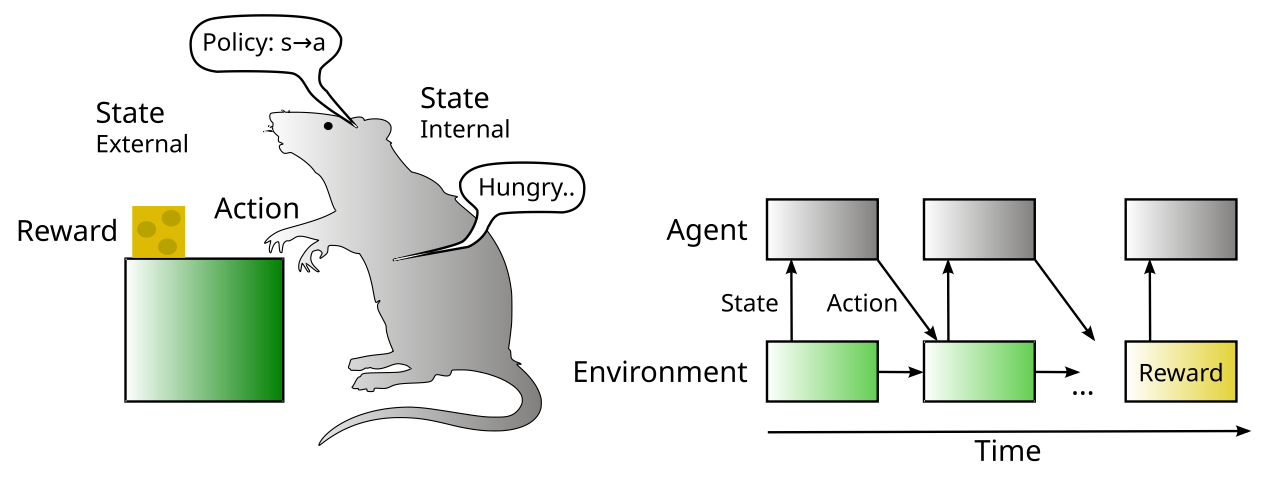
Figure 1: Elements of the reinforcement learning framework: The Environment provides States to the Agent over time, which in turn takes Actions that influence the state evolution. Rewards (and punishments) are delivered by the Environment under specific conditions, and the Agent’s presumed job is to learn to take Actions that optimize the receipt of reward (and minimize punishments) over time. Learning the direct mapping of State → Action according to a learned Policy is known as model-free RL. Most RL models largely ignore the internal state of the agent itself, despite its obvious importance in shaping animal behavior.

The major elements of an RL model are shown in Figure 1, in the context of a rat agent that takes actions in an environment that delivers specific state values (via sensory perception for the rat), and which evolves over time under its own dynamics, under the influence of the agent’s actions. The environment also delivers rewards (and punishments), and the standard objective of RL is to learn how to take actions that optimize the receipt of rewards over time.

The strategy for selecting actions can be usefully categorized into two different approaches, which can be thought of in terms of poles along a continuum (where this continuum is actually a high-dimensional space!):

• Model-free: learns a policy that is a direct mapping from states to actions, i.e., stimulus \(\rightarrow\) response (S-R) learning.

• Model-based: uses internal models of the environment in addition to direct sensory experience of the environment, to select actions according to a plan that is based on the model (Figure 2).

From a psychological perspective, this can be thought of as a distinction between habit-based responding vs. a more thoughtful, considered basis of responding, which has been a central focus of theorizing for many years. For example, Thorndike’s law of effect (Thorndike, 1898), which is the central idea behind instrumental conditioning, holds that any action that leads to a positive outcome will be increased in probability (and vice-versa for punishments). This is basically model-free RL, and it has long been associated with the function of the basal ganglia and the role of dopamine for shaping learning in this brain area (but not perhaps entirely accurately).

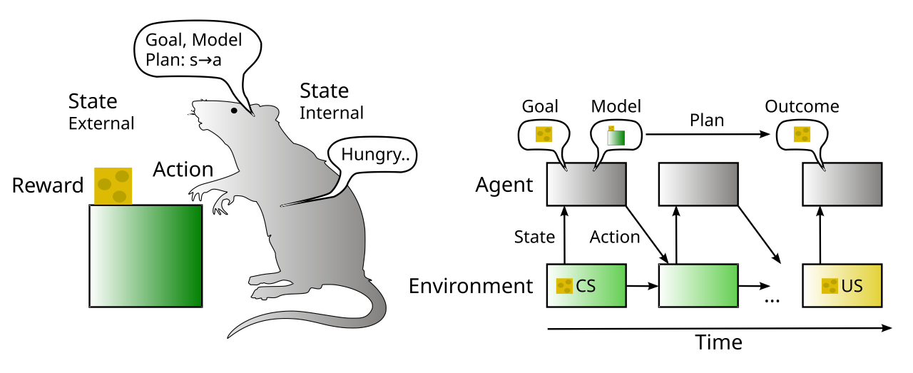
Figure 2: Model-based RL adds internal Goals, Models, and Plans to the basic RL paradigm, so that action selection can be based on internal representations of the possible outcomes of actions, not just learned stimulus-response associations. The CS (conditioned stimulus) can trigger activation of internal Goals to obtain the associated US (unconditioned stimulus) outcome, using an internal Model of the environment to develop a Plan of action to do so.

By contrast, goal-directed or controlled processing (Tolman, 1948; Balleine & Dickinson, 1998; Shiffrin & Schneider, 1977; Cohen et al., 1990; Miller & Cohen, 2001) characterizes the more considered mode of processing, where possible consequences of an action are actually evaluated, instead of just responding on the basis of stimulus-response learning. This mode of processing typically depends on the prefrontal cortex, which has the ability to maintain and manipulate internal representations (of possible actions and their consequences) in a way that is not generally possible in posterior neocortex. This distinction was also popularized by Kahneman (2011) in terms of system 1 (fast) vs. system 2 (slow).

The direct mapping of the RL model-free vs. model-based concepts onto these biological and psychological terms, as initially proposed by Doya (1999) and Daw et al. (2005), has a number of issues that we will encounter in the context of the Rubicon model (O’Reilly et al., 2020). Nevertheless, conceptually all of these different terminologies are generally capturing similar intuitive ideas, which we can all relate to in terms of our daily experiences.

Terminologically, Figure 2 illustrates the main terms from the animal learning, conditioning literature:

• US: unconditioned stimulus. This is a biologically special outcome stimulus such as food or water that requires no learning to recognize as valuable. The US generates the reward scalar value that drives RL, but the two are not equivalent. For example, if not hungry, then food may not be rewarding. Furthermore, one might be craving a particular type of food, such that a different one is not rewarding (and the particular taste of a specific instance can play a big role as well). Most RL models elide these additional levels of complexity, but the Rubicon model includes them, with multiple levels of outcome representations, along with drives such as hunger etc.

• CS: conditioned stimulus. This is an initially arbitrary stimulus that has a reliable predictive association with a US, such that the experience of this stimulus can activate an expectation of that US. These elements of the environmental state are the primary drivers of reinforcement learning, to drive actions needed to obtain the US.

In the model-free context, the CS is the S stimulus in S-R learning. In the model-based context, it is a trigger to activate a goal / plan representation that organizes behavior to obtain the US. The RL framework provides precise definitions and equations for these distinctions, which we will summarize in the following sections. Interestingly, even though model-based RL should in principle be more powerful than model-free, the additional complexities involved actually make it rather difficult to demonstrate advantages in practice, and many of the state-of-the-art models are much closer to the model-free end of the spectrum (Moerland et al., 2021; Plaat et al., 2023). The reasons for this are explained initially in the next section, and then in more detail later.

The curse of dimensionality

The process of trial-and-error learning inevitably requires a serial, step-by-step sequence of actions to achieve a consequent reward. The serial nature of this process makes it particularly strongly subject to the curse of dimensionality: as there are more possible actions and the complexity of the state space increases, the size of the overall space explodes exponentially, quickly making it impossible for a single individual to explore much of this space in their own lifetime. Fundamentally, there is no “free lunch” way out of this problem: finding good solutions to problems ultimately reduces to a form of search through a combinatorially huge space.

There are two fundamental ways to combat this problem:

1. Reduce the size of the space. This is essentially the strategy that symbolic AI models and many current RL models take, by focusing on games like chess and video games, where the overall search space can be constrained, often involving significant domain-specific knowledge about the problem (coming “magically” from outside the scope of an individual agent’s learning experience).

A more generally applicable version of this approach is known as shaping, where a larger overall problem space is initially compressed into a much smaller, simpler space, in a way that can then be gradually expanded to encompass the much larger, richer space of interest. The educational curriculum is specifically designed in this way, with a long sequence of foundational building blocks that lead up to high levels of overall capability in complex, real-world problem spaces. Early learning in human development benefits from “starting small”, with limited memory, perceptual and motor capacities reducing the size of the search space (Newport, 1990; Elman, 1993; Thompson-Schill et al., 2009; Yu et al., 2007).

2. Use efficient (polynomial time) search algorithms: by using dedicated-weight state representations and gradient-based algorithms, one can actually fight dimensionality with dimensionality! There are a number of different manifestations of this approach:

• Dedicated-parallel, gradient-based search in a planning process prior to acting, via constraint satisfaction and optimized representations more generally. In short, if you can use efficient search algorithms to rapidly find “reasonable” coherent plans to then explore through actual serial behavioral trial-and-error exploration, the effective search space can be dramatically reduced in size. Note that this planning process results in an effective compression of the space, unifying both of the above solutions.

• Dedicated-parallel, gradient-based search through the online action control space, by using distributed representations of actions, with graded dynamics so that meaningful gradients can be explored in parallel instead of serially by picking one discrete action at a time. This is what the dorsolateral motor areas of the basal ganglia appear to be doing. This goes hand-in-hand with gradient-based learning in state abstraction to create a more compact, efficient representation of the state, thereby reducing the overall dimensionality of the space.

• Evolution is effectively a highly parallel search algorithm over the space of genomes and organisms to find those that maximize survival and reproduction as discussed in neural biases.

• Cultural evolution and culture-based learning (e.g., the educational system) represent another important form of parallel search, where each individual in a society, across time, searches though different parts of the overall space, and then can share back with everyone else what they have discovered. The many celebrated advances across math, science, and the humanities that we all learn about in school provide an incredibly advanced foundation for further learning, compared to what an individual by themselves “in the state of nature” would be able to discover. Of course, all of this depends critically on language, and large language models clearly demonstrate how much can be learned in this way. It also depends on social drives that motivate us to share and learn from others.

Thus, it is clear that the human brain tackles the curse of dimensionality problem in an “all of the above” manner, which is likewise the approach we take in Axon and Rubicon. These solutions don’t precisely align with standard model-based vs. model-free distinctions in RL, but the term “model” does show up in several places. In any case, we can usefully shape our understanding of the space of RL models using this distinction, starting with the simpler model-free approach.

Model-free

From an abstract mathematical perspective, RL can be formulated as a markov decision process (MDP), which just means that there are discrete states \(S\) that evolve over time according to a unitary (normalized) transition matrix \(T\) that determines the probability of any given future state, based on the current state and any action taken by the agent. See Sutton & Barto, 1998 for the definitive textbook treatment.

The temporal differences (TD) algorithm provides a mechanism for learning to optimize expected reward in this context, and is one of the most central abstract learning rules used in RL (Samuel, 1959; Sutton & Barto, 1981; Sutton, 1988; Sutton & Barto, 1998). Furthermore, it provides a remarkably accurate explanation for many of the firing properties of dopamine neurons in the ventral tegmental area (VTA) of the brainstem (Montague et al., 1996; Schultz et al., 1997).

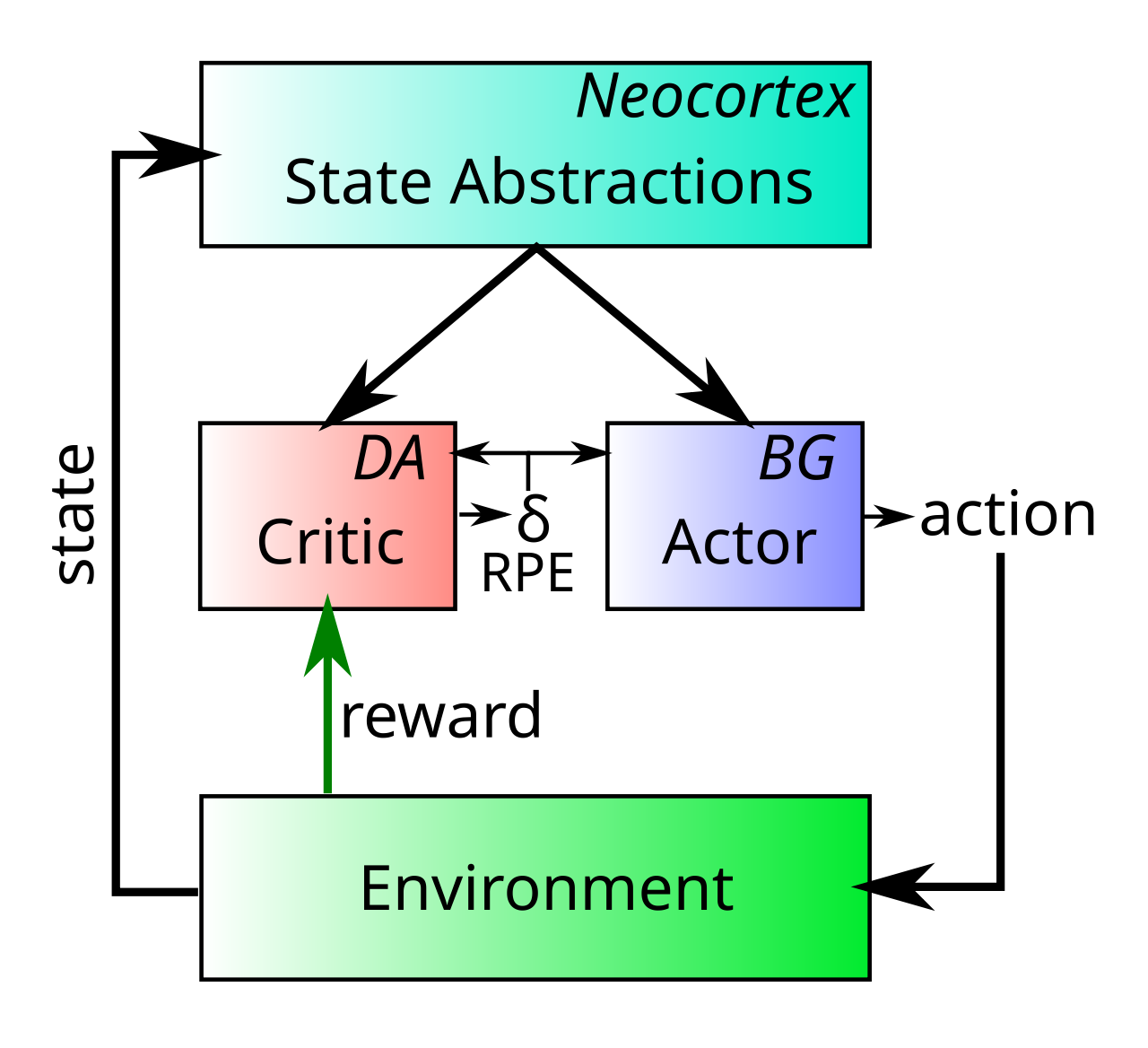
Figure 3: The actor-critic architecture, where the reward prediction error (RPE) signal from the critic is used to train both the critic itself, and the actor system that generates motor actions, which to reward signals from the environment.

Specifically TD provides a way of computing the reward prediction error (RPE) signal in terms of the difference between predicted and actual reward outcomes. In the actor critic architecture (Barto et al., 1983), this RPE signal is generated by the critic, which provides the training signal for improving both motor actions taken by the actor to obtain reward, and the accuracy of the critic’s reward predictions. This is consistent with considerable neuroscience data showing that dopamine modulates learning throughout the brain, especially in the basal ganglia which has both actor and critic functionality.

Reward prediction error

We start with the simplest, highly influential model of reward prediction error, the Rescorla-Wagner conditioning model Rescorla & Wagner, 1972, which is mathematically identical to the delta rule (see error-backpropagation).

The RPE \(\delta\) is just the difference between the actual (\(r\)) and expected (\(\hat{r}\) reward:

\[ \delta = r - \hat{r} \]

In a neural network, this expected reward \(\hat{r}\) can be computed by synaptic weights from sensory input units:

\[ \delta = r - \sum x w \]

The weights can learn to accurately predict the actual reward values, and this delta value specifies the direction in which the weights should change:

\[ \Delta w = \delta x \]

This is identical to the delta learning rule, including the important dependence on the stimulus activity x — you only want to change the weights for stimuli that are actually present (i.e., non-zero x’s).

When the reward prediction is correct, then the actual reward value is canceled out by the prediction, as shown in the second panel in Figure 1 in dopamine. This rule also accurately predicts the other cases shown in the figure too (positive and negative reward prediction errors).

However, what the Rescorla-Wagner model fails to capture is the firing of dopamine to the onset of the CS in the second panel in Figure 1.

TD

In this context, the TD algorithm captures CS-onset firing by introducing time into the equation (as the name suggests) (Sutton & Barto, 1981; Sutton & Barto, 1998). Relative to Rescorla-Wagner, TD just adds one additional term to the delta equation, f, representing the future reward values that might come later in time:

\[ \delta = (r + f) - \hat{r} \]

Now the reward expectation \(\hat{r}=\sum x w\) has to try to anticipate both the current reward r and this future reward f. In a simple conditioning task, where the CS reliably predicts a subsequent reward, the onset of the CS results in an increase in this f value, because once the CS arrives, there is a high probability of reward in the near future. Furthermore, this f itself is not predictable, because the onset of the CS is not predicted by any earlier cue (and if it was, then that earlier cue would be the real CS, and drive the dopamine burst). Therefore, the r-hat expectation cannot cancel out the f value, and a dopamine burst ensues.

Although this f value explains CS-onset dopamine firing, it raises the question of how can the system know what kind of rewards are coming in the future? Like anything having to do with the future, you fundamentally just have to guess, using the past as your guide as best as possible. TD does this by trying to enforce consistency in reward estimates over time. In effect, the estimate at time t is used to train the estimate at time t+1, and so on, to keep everything as consistent as possible across time, and consistent with the actual rewards that are received over time.

This can all be derived in a very satisfying way by specifying something known as a value function, V(t) that is a sum of all present and future rewards, with the future rewards discounted by a gamma factor, which captures the intuitive notion that rewards further in the future are worth less than those that will occur sooner. As the Wimpy character says in Popeye, “I’ll gladly pay you Tuesday for a hamburger today.” Here is that value function, which is an infinite sum going into the future:

\[ V(t) = \left. r(t) + \gamma^1 r(t+1) + \gamma^2 r(t+2) ... \right. \]

We can get rid of the infinity by writing this equation recursively:

\[ V(t) = \left. r(t) + \gamma V(t+1) \right. \]

And because we don’t know anything for certain, all of these value terms are really estimates, denoted by the little “hats” above them:

\[ \hat{V}(t) = r(t) + \gamma \hat{V}(t+1) \]

So this equation tells us what our estimate at the current time t should be, in terms of the future estimate at time t+1. Next, we subtract V-hat from both sides, which gives us an expression that is another way of expressing the above equality — that the difference between these terms should be equal to zero:

\[ 0 = \left( r(t) + \gamma \hat{V}(t+1) \right) - \hat{V}(t) \]

This is mathematically stating the point that TD tries to keep the estimates consistent over time — their difference should be zero. But as we are learning our V-hat estimates, this difference will not be zero, and in fact, the extent to which it is not zero is the extent to which there is a reward prediction error:

\[ \delta = \left( r(t) + \gamma \hat{V}(t+1) \right) - \hat{V}(t) \]

If you compare this to the equation with f in it above, you can see that:

\[ f = \gamma \hat{V}(t+1) \]

and otherwise everything else is the same, except we’ve clarified the time dependence of all the variables, and our reward expectation is now a “value expectation” instead (replacing the r-hat with a V-hat). Also, as with Rescorla-Wagner, the delta value here drives learning of the value expectations.

The TD learning rule can be used to explain a number of different conditioning phenomena, and its fit with the firing of dopamine neurons in the brain has led to a huge amount of research progress. It represents a real triumph of the computational modeling approach for understanding (and predicting) brain function.

From a neuroscience perspective there are actually a number of different brain areas and circuits that work together to drive the firing of VTA dopamine neurons, as summarized in the PVLV model (O’Reilly et al., 2007; Hazy et al., 2010; Mollick et al., 2020). These mechanisms produce some important differences in dopamine firing behavior relative to the predictions of the TD model, including critically the absence of a chain-like progression of firing at the time of the US to the time of the CS, among others (Mollick et al., 2020). Nevertheless, the TD model provides an elegant and computationally powerful learning framework that explains many critical aspects of the role of dopamine in learning across different brain areas.

TD versus temporal derivative learning

Although they share some core conceptual similarities, and a very similar name, it is important to distinguish the TD framework from the temporal derivative based learning mechanisms used in Axon for error-driven learning in the neocortex, via the kinase algorithm. Most importantly, from a biological perspective, TD translates a temporal difference signal into the firing of dopamine neurons, which then explicitly represents the RPE signal. By contrast, the prediction error signal in the temporal derivative framework remains implicit as a difference in neural activity over time, which propagates throughout the neocortex via bidirectional connectivity. Each synapse then adjusts its synaptic weights locally in a way that is sensitive to these temporal derivatives, as contrasted with the direct neuromodulatory role played by dopamine.

Model-based

Many different model based mechanisms can be used in addition or instead of model-free RL (Moerland et al., 2021; Plaat et al., 2023). Many of these mechanisms have direct analogs in the cognitive and neuroscience domain, and are useful for providing a computational insights into these areas. As will become apparent, each of these approaches has clear intuitive advantages, but also significant computational challenges that often prevent these advantages from being realized in more realistic, complex task domains.

The root of most of these challenges is none other than the curse of dimensionality as discussed above. Specifically, many of the standard model-based RL approaches are based on serial search through the space of different possible models, plans, or goals, which quickly becomes intractable as the dimensionality of the relevant space increases. This issue, together with the increased complexity of the models themselves, is why model-based approaches tend to underperform more model-free approaches, which can get away with a more “brute force”, big-data learning solution to specific, well-defined problems.

However, it is clear that the model-free approach will never lead to a truly flexible system that can generalize effectively to novel environments and problems, because it just learns a direct policy of action, without the necessary abstractions and mechanisms needed to adapt to these novel situations.

Thus, to make the model-free approach live up to its theoretical potential, the solutions discussed earlier need to be applied: various ways of compressing the overall search space, including an evolutionary foundation upon which learning builds, and using parallel search algorithms that scale effectively (on parallel hardware such as the brain) to high-dimensional spaces.

The parallel constraint satisfaction via bidirectional connectivity in Axon can dynamically activate optimized representations that effectively search high-dimensional spaces and reduce them to much simpler, lower-dimensional abstractions. These smaller spaces can then be operated upon sequentially within the evolutionarily based Rubicon goal-driven system, that provides strong biases on how to most effectively search the space by conservatively choosing the best immediate goals to pursue, and shaping learning to provide the appropriate information for making these decisions.

With all of this in mind, some of the specific approaches that fall under the model-free umbrella are discussed below.

State abstraction

Instead of directly using the raw state inputs, higher-level abstractions often provide a better basis space for deciding which actions to take. The importance of this computational principle is discussed at length in categorization and generalization, and many critical aspects of human intelligence depend on powerful abstractions performed in the posterior neocortex. In effect, our brains provide us with a rich and complex internal model of the world, at many different levels of abstraction.

The deep layered architectures of abstract neural networks enable these kinds of abstractions to develop, and the marriage of such architectures with reinforcement learning has led to impressive performance on challenging tasks such as playing a wide variety of games, from Atari video games to classics such as chess and go (e.g., Silver et al., 2016). A paradigmatic example is the Deep Q-learning Network (DQN) (Mnih et al., 2015), which couples a deep convolutional network (DCN) with TD-style Q-learning as described above, using “end-to-end” error backpropagation to train representations across many network layers, which are thus specifically optimized for action selection and reward prediction.

One of the key insights from the DQN models is that the sequential nature of trial-and-error learning drives strong positive feedback loops when trained in an online manner, which can be mitigated by randomly reshuffling the order of learning relative to actual experience (Lin, 1992). Although Mnih et al. (2015) cited biological inspiration from the hippocampus for this mechanism, this is not actually very plausible, as most forms of RL learning are preserved in people with hippocampal lesions (e.g., Corkin, 2002). Thus, this issue remains as an important challenge to be solved for our biologically based approach.

Predictive learning of internal models of the environment can generate compact, systematic, combinatorial representations that provide a lower-dimensional basis for generating actions. The powerful internal representations in large language models trained on predictive learning are a good example of this approach, and provide a nice model of the kinds of deep semantic knowledge that humans learn in the neocortex.

To the extent that state abstraction depends on parallel gradient-based learning, it can avoid the curse of dimensionality, and is thus a well-established and essential element of many successful RL models.

World models

The notion of a world model, which is widely discussed in the robotics field, extends the idea of state abstraction to include temporal dynamics, which can approximate the MDP transition matrix of the environment, in formal terms. Thus, such models can potentially be used for mental simulation or imagination of different possible courses of action, which is the original definition of model-based RL. An early paradigmatic example of this is the Dyna architecture of Sutton (1991), which uses a learned transition matrix function to generate synthetic training data to accelerate the learning process.

A world model is also known as a forward model of the environment Jordan & Rumelhart, 1992, and it is essentially what predictive learning does: learning to predict what will happen next. As we discussed extensively in that page, predictive learning is essentially “free” when you have sequential structure in an environment, and this is what enables large language models to train on so much textual data. Thus, we assume that a major component of the posterior neocortical learning is learning these kinds of dynamical, predictive, forward models of the world.

Recent examples of such models include the various Dreamer networks (Hafner et al., 2022; Hafner et al., 2018), which do multi-step roll-outs of predicted sequences of events using learned world models in the context of various video-game based environments. These roll-outs can then anticipate the future consequences of possible action choices, potentially enabling better decision-making.

However, a major issue with such models is that any inaccuracies will compound exponentially over iterated time steps, and typically the environment is sufficiently stochastic that the branching factor for different possible future “timelines” also grows exponentially (recent Marvel-universe movies capture this problem nicely). Thus, this approach quickly breaks down under the curse of dimensionality in the state space, as a function of time and complexity within any given state.

Multiscale models

The longstanding principle of hierarchical, multi-scale representations (e.g., Barto & Mahadevan, 2003) can potentially help with the above problems in world models, by performing predictions at more abstract, coarse-grained levels where the dimensionality is sufficiently low, and the stochasticity is encapsulated in the abstractions instead of being directly manifest in the dynamics. This is a key element of the Rubicon model.

Hierarchical approaches to RL encompass the concept of subgoals: breaking a complex problem down into more manageable sub-tasks, as in the widely discussed options framework in RL (Sutton et al., 1999), and the chunking mechanism in the ACT-R framework (Anderson & Lebiere, 1998). The difficulty with these and related hierarchical RL approaches is that it is often hard to know when and how to organize relevant subtasks, and the possibilities for the number of ways to do so is again subject to exponential combinatorial explosion problems (Pateria et al., 2021). Thus, we are not optimistic that various heuristic mechanisms for shaping task and plan representations will scale up to more complex real-world cases (Collins & Frank, 2013; Schapiro et al., 2013).

Furthermore, almost everywhere any kind of rigid hierarchical system has been proposed, one quickly realizes that the real world is not actually so amenable to such systems, and requires more graded, flexible, soft frameworks (e.g., Rogers & McClelland, 2004).

Planning mechanisms

There is a large literature on planning algorithms, which converges in many cases with approaches used in the RL world (Russell & Norvig, 2016; Moerland et al., 2021). Intuitive ideas include searching forward from the current state to try to find a desired outcome, versus searching backward from the desired outcome state to find a path that connects to the current state. In every case, the planning process requires something like a world model that allows the different possible actions to be simulated in order to search through the space.

The human-beating AI approaches to the games of chess and go relied on these classical-style state-space planning algorithms, constructed using domain-specific knowledge about the rules and relevant structure of these games in order to combat the severe combinatorial explosion problems (Silver et al., 2016; Silver et al., 2017). Thus, despite the success of these specific examples, they fail to generalize to more complex real-world tasks, which lack the ability to leverage domain-specific knowledge needed to search the problem space.

Consistent with the overall solutions to these combinatorial explosion problems discussed above, it seems clear that planning must occur in parallel, and this is precisely what the parallel constraint satisfaction process is known to be effective at doing. Instead of serially searching in one direction or another, this process searches in parallel for plans that are consistent with both the starting and target outcome states, along with any number of other constraints available from the environment, in terms of the shape of the space, tools or other artifacts available, etc.

Exploration vs. exploitation

The RL framework exposes a fundamental tradeoff between exploring new action plans and areas of the environment to potentially obtain greater reward, versus exploiting what has already been learned to optimize reward by making the currently optimal choices. We experience this tradeoff every time we choose between trying a new restaurant, or a new item on the menu, versus going with the established favorites. Interestingly, there are individual differences in these behaviors, associated with stable personality traits such as openness to new experiences, suggesting that there is no single best solution (that’s why it is a tradeoff), with variation across the population being beneficial to cover all the bases. Some people take risks and make great new discoveries, while others ensure that established rewards are properly reaped.

Age also plays a critical role in the balance between exploration and exploitation, with more exploration needed when young to discover what works across a broader range of the space, while older individuals can safely rely more on their accumulated wisdom. This shifting balance can happen naturally in an RL system as the learning proceeds, when action selection is based on learned weights that start out small and equivocal: as these become stronger and more sharply tuned, behavior naturally becomes more determined by the existing weights. Additional hyperparameters may also be adjusted to shift this balance as well.

For example, the notoriously risky behavior of adolescents has been attributed to a heightened exploration bias, before settling down and becoming a boring old adult (Casey et al., 2008). Changes in the levels of dopamine neuromodulation have been attributed to this shift (Spear, 2000).

The Rubicon model includes a novelty bias that induces exploration when there aren’t other learned options available, and it also updates internal drive states, so that satiety can drive further exploration. Furthermore, Rubicon implements exploration at the level of overall goal states, rather than in terms of each individual action step, which is critical for supporting a more strategic exploration strategy (Ecoffet et al., 2021).