Linear algebra

The language of linear algebra provides an important set of concepts for understanding the behavior and learning in neural networks, and also important analysis techniques including linear regression and principal components analysis. See also information theory for a similarly useful framework.

For example, the state of activity in a network layer can be thought of as an n-dimensional vector of numbers representing the activity of each of the n neurons in the layer. We can write this vector using bold lower-case letters, with x being the input layer and y (of dimension m) being the hidden layer above that. The set of weights interconnecting the two layers, W, is thus an n x m matrix (confusingly, n = number of columns, m = number of rows, but indexes are written in the opposite order).

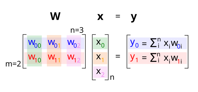
Figure 1: Matrix multiplication of n=3 vector of input-layer activations x, by n x m matrix of weights W, gives the linear activity of m=2 hidden-layer activations y. Matrix multiplication is tricky because it generally operates on the right and is not commutative, so the order matters. x and y are represented as column vectors to make everything work correctly. As coded by the colors, the first hidden unit in y is computed as the dot product of the first row of the weight matrix, with each column applying to a different input unit in turn. The index i is used conventionally for the input layer in neural networks, but typically in linear algebra this would be a j for the column-wise variable of a matrix.

Figure 1 shows how the matrix multiplication of the input vector x times the weight matrix W gives the linear activations of the hidden layer neurons, as in the following equation:

\[ {\bf y} = {\bf W} {\bf x} \]

Each row of the weight matrix W contains a vector of weights for each receiving neuron in the hidden layer, and the operation of matrix multiplication is just the accumulation of the individual dot product (sum of element-wise products) multiplications of these two vectors:

\[ y_j = \sum_i^n x_i W_{ji} \]

This dot product should be familiar from the neuron chapter section on Computing input conductances, and biologically corresponds to the total conductance caused by AMPA excitatory channels opening in response to the rate of sending neuron spiking (and thus glutamate neurotransmitter release), with the weight value corresponding to the number and efficacy of these AMPA receptors at each synapse.

Dot products are projections

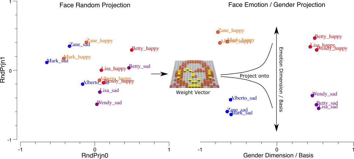
Figure 2: How synaptic weights act to project input patterns along specific dimensions or bases, in this case projecting the inputs along the dimensions of Emotion and Gender. In the left panel, the very high-dimensional face inputs (256 dimensions for a 16x16 image) are projected along two random weight vectors, allowing us to visualize this high-dimensional input space in a 2D plot. In the right panel, the specific synaptic weights trained for discriminating along the emotion vs. gender dimensions have transformed or rotated the input space into a much more systematic and well-organized, low-dimensional space. This is fundamentally what neurons do: organize and transform input patterns along relevant dimensions, and that is another way of stating that neurons detect stimuli along these dimensions.

The dot product operation (also known as the inner product or scalar product) takes two vectors and turns them into a single scalar number representing the extent to which the two vectors “align” with each other. This is known as a projection computation in linear algebra terms: you are effectively seeing one vector “through the lens” of the other vector. Thus, the receiving neuron sees the input vector “through the lens” of its synaptic weights for that input layer, as explored in the detector simulation. Anywhere there are zero values in the weights, the input values are “filtered out” and are irrelevant, while strong weights make those inputs highly important for driving the receiver’s activity.

Figure 2 illustrates this projection operation in the context of the faces simulation, as discussed in categorization. This projection operation organizes and systematizes the inputs along dimensions of behavioral importance, for example projecting a face input along dimensions of emotion and gender in the case shown in the figure, which you can explore in the faces simulation.

Basis space

Another linear algebra framing of this operation is in terms of the synaptic weight matrix being composed of basis vectors, where each row of the matrix defines a different basis or axis of a new, rotated version of the space defined by the the input activity vector. Thus, the hidden layer neurons are creating a transformation of the input space into this new rotated space, which amplifies certain things while filtering out others.

Furthermore, this basis space can help with the curse of dimensionality by using fewer basis vectors to capture most of the important dimensions of variance, relative to the high dimensionality of the original space. For example, original dimensions that are largely redundant (e.g., the shapes of the eyes and the mouth used in expressing different emotions) can be combined together into one basis vector.

Eigenvectors

The process of principal components analysis (PCA) provides a way of selecting a new set of basis vectors to project the input space into, based on the linear algebra process of eigenvector decomposition, where the eigenvector is a special vector that keeps pointing in the same direction when multiplied by the matrix that it is an eigenvector of:

\[ {\bf A}{\bf v} = \lambda {\bf v} \]

where A is a matrix, and v is an eigenvector of that matrix because its multiplication produces the same vector again, scaled by a scalar value \(\lambda\) which is the associated eigenvalue for that eigenvector v.

The eigenvectors with the largest eigenvalues provide the most “information” about matrix A, and thus a typical use of PCA is for dimensionality reduction to represent a much higher dimensional space in terms of its strongest 2 eigenvectors, which can then be plotted in a 2D plot. Otherwise, visualizing large n-dimensional spaces can be hard.

Interestingly, Hebbian learning can be shown mathematically to be performing PCA, providing a powerful conceptual understanding of what it might be doing: learning new efficient ways of representing the input activity space.

Least squares regression

One of the most basic problems in linear algebra is to solve the least squares problem:

\[ \rm{minimize} \; \|{\bf W} {\bf x} - {\bf t}\|^2 \]

which means finding the values of the matrix W that minimizes the differences between target activation values t and the y activation values that the network computes (using Eq 1), across all of the relevant input activation states of x. This is the problem that linear regression solves, and is another way of expressing the basic goal of error-driven learning, and error backpropagation provides an iterative solution to this same problem in a two-layer linear network of this form.

Thus, two major forms of neural network learning, Hebbian and error-driven, can be understood in simple, essential form using the tools of linear algebra.

Non-negative factorization

There are important constraints that arise by requiring a basis space to be encoded using only positive-valued numbers (i.e., non-negative factorization; Lee & Seung, 1999). Because neurons can generally only have positive-only weights from a given sending neuron, and they also only send positive-valued signals in terms of rates of spiking, this non-negative space is important for understanding the impact of these constraints relative to abstract neural network models lacking such constraints.

Intuitively, thinking in terms of the weights shown in Figure 1, if each weight value must be non-negative and the weight vectors must be orthogonal to each other (i.e., to encode independent factors), then there can be no overlapping weight values in a given column. For a complete basis representation of a 3D space, i.e., 3 such weight vectors (only 2 are shown in the figure), this would mean that each weight must have a 1 in one unique column, and a 0 in each of the other two columns.

Thus, the non-negativity constraint is much stronger than the orthogonality constraint by itself (which is all that PCA imposes), effectively uniquely determining the basis vectors to be simple localist encodings of the original input dimensions (where each row of the x input vector is a different input dimension). By contrast, infinitely many orthogonal basis vectors with negative elements can be constructed, as different rotations of the original input dimensions. Critically, a rotation requires both positive and negative numbers: whatever is added to one dimension must be taken from the others, and that zero-sum nature of a rotation implies the requirement for both signs.

If there is a much larger space of input dimensions than basis vectors, then the non-negative constraint still tends to impose a more sparse representation that has significant weighting on relatively few input dimensions, because they still cannot overlap with each other and remain orthogonal. As with the localist case, the non-negativity constraint thus forces the basis vectors to align directly with the original input dimensions – these input dimensions represent a privileged basis under the non-negativity constraint, whereas they are not otherwise privileged without that constraint.

See quantum-analogies for a further exploration of the relationship between non-negative factorization versus sign-unconstrained factorization (e.g., PCA) and the differences between standard “classical” probabilities versus quantum probabilities, and the broader implications of quantum-level phenomena for understanding aspects of how the brain works.