
Neuron bayesian
This page shows how the neuron equilibrium potential equation, derived based on the biology of the neuron, can also be understood in terms of Bayesian hypothesis testing (Hinton & Sejnowski, 1983; McClelland, 1998). In this framework, one is comparing different hypotheses in the face of relevant data, which is analogous to how the detector is testing whether the signal it is looking for is present (\(h\)), or not (\(\overline{h}\)). The probability of \(h\) given the current input data \(d\) (which is written as \(P(h|d)\)) is a simple ratio function of two other functions of the relationship between the hypotheses and the data (written here as \(f(h,d)\) and \(f(\overline{h},d)\)):
\[ P(h|d) = \frac{f(h,d)}{f(h,d) + f(\overline{h},d)} \]
Thus, the resulting probability is just a function of how strong the support for the detection hypothesis \(h\) is over the support for the null hypothesis \(\overline{h}\). This ratio function may be familiar to some psychologists as the Luce choice ratio used in mathematical psychology models for a number of years.
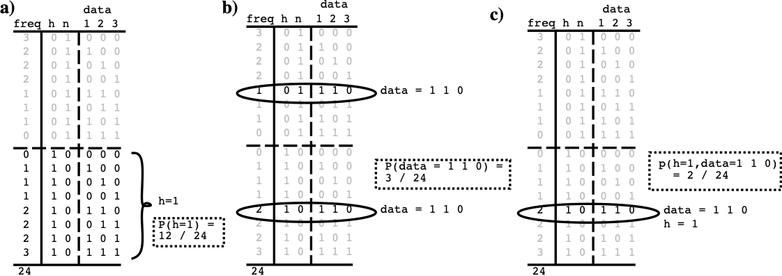
Figure 1: Simple example data to compute probabilities from, for line detecto — just add up number of cases where a given condition is true, and divide by the total number of cases (24): a \(P(h=1) = <sup>12</sup>⁄<sub>24</sub> = .5\). b \(P(d=1 1 0) = <sup>3</sup>⁄<sub>24</sub> = .125.\) $\(c** \)P(h=1, d=1 1 0) = 2⁄24 = .0833.$
To have a concrete example to work with, consider a detector that receives inputs from three sources, such that when a vertical line is present (which is what it is trying to detect), all three sources are likely to be activated (Figure 1). The hypothesis \(h\) is thus that a vertical line is actually present in the world, and \(\overline{h}\) is that it is not. \(h\) and \(\overline{h}\) are mutually exclusive alternatives: their summed probability is always 1. There are three basic probabilities that we are interested in that can be computed directly from the world state table — you just add up the number of cases where a given situation is true, and divide by the total number of cases (with explicit and complete data, probability computations are just accounting):
• The probability that the hypothesis \(h\) is true, or \(P(h=1)\) or just \(P(h)\) for short = 12⁄24 or .5.
• The probability of the current input data, e.g., \(d=1 1 0\), which is \(P(d=1 1 0)\) or \(P(d)\) for short = 3⁄24 (.125) because it occurs 1 time when the hypothesis is false, and 2 times when it is true.
• The intersection of the first two, known as the joint probability of the hypothesis and the data, written \(P(h=1, d=1 1 0)\) or \(P(h,d)\), which is 2⁄24 (.083).
The joint probability tells us how often two different states co-occur compared to all other possible states, but we really just want to know how often the hypothesis is true when we receive the particular input data we just got. This is the conditional probability of the hypothesis given the data, which is written as \(P(h|d)\), and is defined as follows:
\[ P(h | d) = \frac{P(h, d)}{P(d)} \]
So, in our example where we got \(d=1 1 0\), we want to know:
\[ P(h=1 | d=1 1 0) = \frac{P(h=1, d=1 1 0)}{P(d=1 1 0)} \]
which is (2⁄24) / (3⁄24), or .67 according to our table. Thus, matching our intuitions, this tells us that having 2 out of 3 inputs active indicates that it is more likely than not that the hypothesis of a vertical line being present is true. The basic information about how well correlated this input data and the hypothesis are comes from the joint probability in the numerator, but the denominator is critical for scoping this information to the appropriate context (cases where the particular input data actually occurred).
The above equation is what we want the detector to solve, and if we had a table like the one in Figure 1, then we have just seen that this equation is easy to solve. However, having such a table is nearly impossible in the real world, and that is the problem that Bayesian math helps to solve, by flipping around the conditional probability the other way, using what is called the likelihood:
\[ P(d | h) = \frac{P(h, d)}{P(h)} \]
It is a little bit strange to think about computing the probability of the data, which is, after all, just what was given to you by your inputs (or your experiment), based on your hypothesis, which is the thing you aren’t so sure about! However, think of it instead as how likely you would have predicted the data based on the assumptions of your hypothesis. In other words, the likelihood computes how well the data fit with the hypothesis.
Mathematically, the likelihood depends on the same joint probability of the hypothesis and the data, we used before, but it is scoped in a different way. This time, we scope by all the cases where the hypothesis was true, and determine what fraction of this total had the particular input data state:
\[ P(d=1 1 0 | h=1) = \frac{P(h=1, d=1 1 0)}{P(h=1)} \]
which is (2⁄24) / (12⁄24) or .167. Thus, one would expect to receive this data .167 of the time when the hypothesis is true, which tells you how likely it is you would predict getting this data knowing only that the hypothesis is true.
The main advantage of a likelihood function is that we can often compute it directly as a function of the way our hypothesis is specified, without requiring that we actually know the joint probability \(P(h,d)\) (i.e., without requiring a table of all possible events and their frequencies). Assuming that we have a likelihood function that can be computed directly, Bayes formula is just a simple bit of algebra that eliminates the need for the joint probability:
\[ P(h, d) = P(d | h) P(h) \]
such that:
\[ P(h|d) = \frac{P(d|h) P(h)}{P(d)} \]
It allows you to write \(P(h|d)\), which is called the posterior in Bayesian terminology, in terms of the likelihood times the prior, which is what \(P(h)\) is called. The prior indicates how likely the hypothesis is to be true without having seen any data at all — some hypotheses are just more plausible (true more often) than others, and this can be reflected in this term. Priors are often used to favor simpler hypotheses as more likely, but this is not necessary. In our application here, the prior terms will end up being constants, which can actually be measured (at least approximately) from the underlying biology.
The last barrier to actually using Bayes formula is the denominator \(P(d)\), which requires somehow knowing how likely this data is compared to any other. Conveniently, we can replace \(P(d)\) with an expression involving only likelihood and prior terms if we make use of the null hypothesis \(\overline{h}\). Because the hypothesis and null hypothesis are mutually exclusive and sum to 1, we can write the probability of the data in terms of the part of it that overlaps with the hypothesis plus the part that overlaps with the null hypothesis:
\[ P(d) = P(h,d) + P(\overline{h},d) \]
In Figure 1, this amounts to computing \(P(d)\) in the top and bottom halves separately, and then adding these results to get the overall result:
\[ P(d) = P(d|h) P(h) + P(d|\overline{h}) P(\overline{h}) \]
which can then be substituted into Bayes formula, resulting in:
\[ P(h|d) = \frac{P(d|h) P(h)}{P(d|h) P(h) + P(d|\overline{h}) P(\overline{h})} \]
This is now an expression that is strictly in terms of just the likelihoods and priors for the two hypotheses! Furthermore, it is this is the same equation that we showed at the outset, with \(f(h,d) = P(d|h) P(h)\) and \(f(\overline{h},d) = P(d|\overline{h}) P(\overline{h})\). It has a very simple \(\frac{h}{h+\overline{h}}\) form, which reflects a balancing of the likelihood in favor of the hypothesis with that against it. It is this form that the biological properties of the neuron implement. You can use the table in Figure 1 to verify that this equation gives the same results (.67) as we got using the joint probability directly.
The reason we cannot use something like the table in Figure 1 in the real world is that it quickly becomes intractably large due to the huge number of different unique combinations of input states. For example, if the inputs are binary (which is not actually true for neurons, so it’s even worse), the table requires \(2^{n+1}\) entries for \(n\) inputs, with the extra factor of two (accounting for the \(+1\) in the exponent) reflecting the fact that all possibilities must be considered twice, once under each hypothesis. This is roughly \(1.1 x 10^{301}\) for just 1,000 inputs (and our calculator gives \(Inf\) as a result if we plug in a conservative guess of 5,000 inputs for a cortical neuron).
In lieu of the real data, we have to fall back on coming up with plausible ways of directly computing the likelihood terms. One plausible assumption for a detector is that the likelihood is directly (linearly) proportional to the number of inputs that match what the detector is trying to detect, with a linear factor to specify to what extent each input source is representative of the hypothesis. These parameters are just our standard weight parameters \(w\). Together with the linear proportionality assumption, this gives a likelihood function that is a normalized linear function of the weighted inputs:
\[ P(d|h) = \frac{1}{z} \sum_i d_i w_i \]
where \(d_i\) is the value of one input source \(i\) (e.g., \(d_i = 1\) if that source detected something, and 0 otherwise), and the normalizing term \(\frac{1}{z}\) ensures that the result is a valid probability between 0 and 1.
The fact that we are defining probabilities, not measuring them, makes these probabilities subjective, as compared to frequencies of objectively measurable events in the world. Nevertheless, the Bayesian math ensures that you’re integrating the relevant information in the mathematically correct way, at least.
To proceed, one could define the following likelihood function:
\[ P(d|h) = \frac{1}{12} \sum_i x_i w_i \]
and similarly for the null hypothesis, which is effectively the negation:
\[ P(d|\overline{h}) = \frac{1}{12} \sum_i (1 - x_i) w_i \]
If you plug these into the Bayesian equation, together with the simple assumption that the prior probabilities are equal, \(P(h) = P(\overline{h}) = .5\), you get the same results we got from the table.
Finally, we compare the equilibrium membrane potential equation:
\[ V_m = \frac{g_e \overline{g}_e E_e + g_i \overline{g}_i E_i + \overline{g}_l E_l} {g_e \overline{g}_e + g_i \overline{g}_i + \overline{g}_l} \]
to the Bayesian formula, where the excitatory input plays the role of the likelihood or support for the hypothesis, and the inhibitory input and leak current both play the role of support for null hypotheses. Because we have considered only one null hypothesis in the preceding analysis (though it is easy to extend it to two), we will just ignore the leak current for the time being, so that the inhibitory input will play the role of the null hypothesis.
Interestingly, the reversal potentials have to be 0’s and 1’s to fit the numerical values of probabilities, such that excitatory input drives the potential toward 1 (i.e., \(E_e = 1\)), and that the inhibitory (and leak) currents drive the potential toward 0 (i.e., \(E_i = E_l = 0\)).
\[ V_m \approx P(h|d)\frac{g_e \overline{g}_e}{g_e \overline{g}_e + g_i \overline{g}_i} \]
\[ V_m \approx \frac{P(d|h) P(h)}{P(d|h) P(h) + P(d|\overline{h}) P(\overline{h})} \]
The full equation for \(V_m\) with the leak current can be interpreted as reflecting the case where there are two different (and independent) null hypotheses, represented by inhibition and leak. Inhibition dynamically changes as a function of the activation of other units in the network, whereas leak is a constant that sets a basic minimum standard against which the detection hypothesis is compared. Thus, each of these can be seen as supporting a different kind of null hypothesis.
Taken together, this analysis provides a satisfying computational-level interpretation of the biological activation mechanism, and assures us that the neuron is integrating its information in a way that makes good statistical sense.