Motor

The motor system in the brain involves many different areas, and in many ways, the entire brain exists in service of producing motor output (Figure 1). For example, Daniel Wolpert has made the point that the sea squirt eats its own brain once it no longer needs to move around. More specific discussion of various aspects of motor control can be found in reinforcement learning, basal ganglia, cerebellum, space, and the Rubicon framework. This page provides a high-level overview of the challenges and solutions for motor control, and some details about the underlying physiology of muscles and how the spinal cord and brainstem provide a systematic basis for motor control.

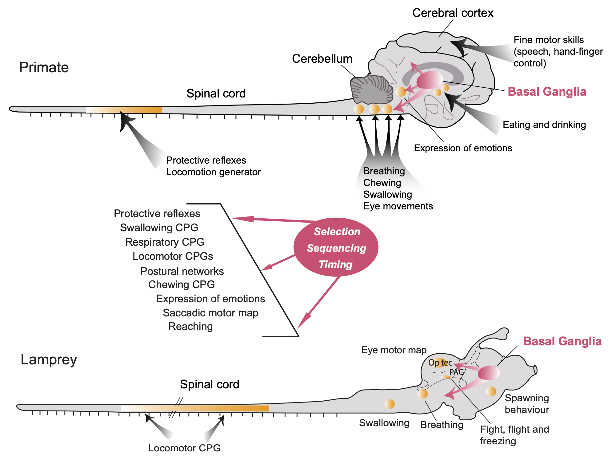
Figure 1: Anatomical organization of the motor system in the lamprey (one of the evolutionarily most ancient vertebrates) and the primate. CPG (central pattern generator) circuits among interneurons in the spinal cord provide a low-dimensional, adaptive (via local proprioceptive and somatosensory feedback) repertoire of muscle synergies that higher levels in the brainstem, cerebellum, basal ganglia, and cerebral cortex control via desceding pathways. The “lamprey core” systems are sufficient for survival, as shown in extensive studies with decorticate cats and other species. From Grillner & El Manira (2020).

Dimensionality reduction, coordination, and muscle synergies

As in all aspects of neural function, the central problem in motor control is managing the curse of dimensionality: there are exponentially many possible combinations of muscle activations over time. How does the brain reduce this huge space down to the relatively small subset of muscle activations necessary to perform the actions needed for an animal’s survival?

This is another instance of the fundamental search problem, and in the case of the motor system, evolution has done a lot of the work by building in complex muscle synergies into the spinal cord and brainstem, where networks of interneurons (excitatory and inhibitory) activate spatiotemporal patterns of muscle activation. From this lower-dimensional repertoire of elements (i.e., a basis space), complex patterns of motor behavior are constructed (Bernstein, 1967; Bernstein, 1996; Tresch et al., 1999; Avella et al., 2003; Ting & McKay, 2007; Bizzi et al., 2008; Tresch & Jarc, 2009; Latash et al., 2010; Ting et al., 2015; Overduin et al., 2015; Takei et al., 2017; Bruton & O’Dwyer, 2018; Latash, 2020; Brambilla et al., 2023).

Another critical problem that is solved by these muscle synergies is the coordination across many different muscles that is required to accomplish any given motor action. The contraction of any given muscle creates a variety of physical consequences for other muscles, including altering the basic center of gravity of the entire organism. Thus, any given action must take all of these consequences into account, and ensure that all of the individual muscle contractions are indeed synergistic, and not working at cross purposes.

A variety of different terms have been used in the literature to refer to these synergies, including reflexes (Sherrington, 1910), central pattern generators (CPGs, Grillner & El Manira, 2020; Grillner & Zangger, 1979), and force fields (Giszter et al., 1993). There are somewhat different connotations of these terms, especially for the CPGs, which apply for example to the complex circuits that drive locomotor behavior, involving sustained, rhythmic, patterned behavior that can extend over long periods of time. More generally, these synergies can be referred to as modules (Bizzi et al., 2008), primitives, building blocks, or components of motor actions.

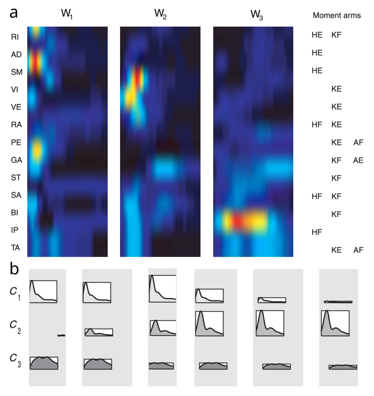
Figure 2: Three muscle synergies extracted from frog kicking behavior. a) Activation of different muscles (vertical axis) over time (horizontal axis), accomplishing given overall motor action (moment arms, aligned by corresponding column order of the synergies): HE hip extension; HF hip flexion; KE knee extension; KF knee flexion; AE ankle extension; AF ankle flexion. b) Activation strengths over time for each synergy component (\(C_{1-3}\)) needed to reconstruct 6 different overall motor actions. These patterns differ primarily in magnitude, not temporal pattern, and indeed the temporal pattern appears to match that of the synergies themselves, suggesting that a more static control signal could accomplish largely the same outcome. From d’Avella et al., 2003

As a concrete example, a detailed analysis of spinal-level muscle synergies in the frog leg system revealed a set of 4 synergies that could be combined with different activation strengths to explain a wide range of overall motor response patterns (Tresch et al., 1999). A subsequent analysis allowing for contributions from the entire brain in intact frogs showed how the timing and activation modulation of 3 different spatiotemporal muscle synergies (Figure 2) can explain this same space of motor responses (Avella et al., 2003).

Thus, the final motor behavior pattern depends on the integrated contributions of multiple levels of control, with the spinal muscle synergies implemented by interneurons providing the lowest level, and higher levels progressively adding their own direct synergies as well as broader coordination across the basic spinal elements (Grillner & El Manira, 2020). For example, an analysis of correlated motor units in hand movement showed last order (i.e., just upstream of the muscle activation) inputs from the pontomedullary reticular formation, the magnocellular red nucleus, and primary motor cortex (M1), in addition to the basic spinal cord interneurons (Xu et al., 2024).

The genetically coded nature of these muscle synergies is evident across many studies showing that the same synergies are found in each of the individual animals studied (e.g., Avella et al., 2003; Bizzi et al., 2008) and they arise early in development and persist into adulthood (Yang et al., 2019), even in humans, where the core patterns in locomotion have strong similarities to those in other species (Dominici et al., 2011). Also, although general-purpose learning mechanisms typically develop low-dimensional basis spaces that resemble muscle synergies (Chai & Hayashibe, 2020; Tresch & Jarc, 2009; Scott, 2004; Todorov & Jordan, 2002), the direct evidence of spinal implementation and strong genetic evidence support the evolutionary basis for these in animals.

Sensory feedback control

The other critical need for dimensionality reduction in the motor system arises from interactions between an animal and its environment, which is also highly variable and thus represents a major additional source of variance and combinatorial explosion. There is considerable evidence that the muscle synergies implemented by spinal cord interneurons incorporate direct feedback control mechanisms, that automatically compensate for environmental perturbations (Wimalasena et al., 2025; Shinohara et al., 2025; Conway et al., 1987; Angel et al., 1996; Alvarez & Fyffe, 2007; Bizzi et al., 2008; Santuz et al., 2019; Gorko et al., 2024). One estimate put the force contribution of these feedback signals at 35% (Stein et al., 2000; Côté et al., 2018).

Unfortunately, the ability to understand these feedback control mechanisms has been impaired by the difficulty in categorizing and mapping the connectivity of the spinal interneurons that process these feedback signals (Sengupta & Bagnall, 2023; McCrea, 1992; Côté et al., 2018). Furthermore, extant circuit-based models only relatively recently began to include such mechanisms (Shinohara et al., 2025 – see Figure 10; Danner et al., 2017). Nevertheless, more abstract state-space analyses of large populations of spinal interneurons have the potential to reveal the presence and dynamical implications of these feedback control mechanisms (Wimalasena et al., 2025).

The rather underdeveloped understanding of feedback control in motor systems contrasts with the theoretical clarity of the mathematically based hierarchical control framework known as perceptual control theory (PCT) (Powers, 1973; Powers, 1973; Cools, 1985; Yin, 2014; Barter & Yin, 2021; Parker et al., 2020). A central premise of this framework is that control should operate on sensory signals, because these sensory signals tell you about the relevant state of the system.

As a simple example, a heating / cooling system (HVAC) should be driven by a target temperature (sensory variable), not a target amount of heat or cooling output (“motor” variable), because the amount of heat or cooling needed obviously depends on the environment. Older cars for example used to only provide control over the HVAC output, relying on the user to make the connection with the desired sensory variables, while more modern cars now have thermostatic control driven by a target temperature, which greatly simplifies the control task.

In short, there are many different combinations of environmental and motor parameters that could be used to accomplish a given action outcome, so exerting control at the level of these motor parameters is underdetermined and inefficient, relative to controlling a sensory variable that is directly connected to the desired outcome.

Empirical demonstrations of PCT show the complete lack of awareness that people have about the actual motor actions they are performing when the motor system is perturbed (Parker et al., 2020). In any case, given the presence of motor synergies at the spinal level, it is already the case that motor control is divorced from individual muscle or joint-based signals (although primate and especially human motor cortex has the ability to provide more fine-grained muscle-level control, as reviewed below).

A closely related and influential theory of motor control is optimal feedback control (OFC) which is likewise based on the principle that online, sensory feedback based control is the only plausible form of control in the face of environmental and other sources of variability (Todorov & Jordan, 2002; Scott, 2004). As in PCT, OFC is based on the principle that control tunes feedback gain parameters, rather than directly driving motor variables such as force.

OFC adds an important connection with computational-level mechanisms of optimization, as useful points of reference, even though biological constraints will likely render the actual system at least somewhat suboptimal in various ways. One consequence of these optimization mechanisms is that they focus only on goal-relevant outcomes (e.g., the temperature in the above example), while ignoring other irrelevant outcomes, which is consistent with empirical data (Vaz et al., 2019).

The uncontrolled manifold (UCM) framework provides a widely used, if confusingly named methodology for identifying the engagement of an optimization mechanism (Scholz & Schöner, 1999; Latash et al., 2007; Latash, 2024). Intuitively, one would expect that the variable that is being controlled by the optimization process (e.g., temperature) would then be associated with a set of underlying parameters that would be labeled something like the controlled parameters (e.g., heat and cooling output levels). However, these are actually the variables within the uncontrolled manifold! Why? Because typically there are multiple different such parameters that could be set in various uncontrolled ways to accomplish the same desired, controlled output.

For example, if there are two different sources of heat (e.g., passive floor heating, which is slow to change, and a fast-changing forced-air vent), then all of the different combinations of these two sources together represent the UCM (where a manifold refers to a constrained subspace within the larger space of all possible parameter values). At any given point, the target temperature can be achieved through some specific combination of these heat sources (e.g., taking into account the current, slowly changing floor heat, and adjusting the forced-air vent as needed). Meanwhile, the cooling sources (and other possible, irrelevant parameters) are all being controlled in the sense of a controlled variable in a scientific experiment: something whose variance is being minimized to ensure it doesn’t interfere with the relevant independent variable being manipulated (where independent is effectively a synonym of uncontrolled in this case).

Despite the confusing name, the UCM framework also captures the key idea that having a full subspace manifold of redundant motor parameters represents an important kind of abundance in motor control (Gelfand & Latash, 1998), where these different parameters can actually be leveraged (one might dare say, controlled) to provide critical flexibility to adapt to novel, complex situations (e.g., carrying multiple things at the same time with different hand configurations, opening doors while carrying something, etc). Thus, instead of regarding the curse of dimensionality as a problem, it is also an opportunity, provided one has a sufficiently powerful, flexible, and dynamic online controller mechanism that can adapt on the fly to all these novel situations. See Latash et al. (2007) for an integration of UCM with the muscle synergies framework, along these lines.

Posture and equilibrium-point control

The PCT framework is consistent with the principle of equilibrium-point motor control, which postulates that descending motor control signals specify a target length for each muscle, rather than dynamical variables such as force (Feldman, 1986; Feldman & Levin, 2009; Gribble et al., 1998; Sainburg, 2015).

One of the compelling advantages of the equilibrium-point model is that it provides a unified framework for understanding the relationship between posture (sitting, standing, etc) and active motor actions. Posture in this context is just a fixed configuration of muscle lengths and joint angles, and action is just the updating of these postural parameters: once the target length is changed, automatic feedback muscle forces would be engaged to transition the system to the new target length. Thus, action is just a change in posture under this framework.

Maintaining a given posture requires persistent ongoing muscle activation. According to the equilibrium-point model, instead of descending control systems having to maintain corresponding active control inputs, it would make more sense for such systems to establish a desired postural configuration, and allow spinal-level circuits driven by relevant feedback mechanisms to maintain this target configuration.

However, once we appreciate that the muscle synergies present in the spinal cord actually do incorporate sensory feedback mechanisms (including muscle length as signalled by the muscle spindle fibers), then the boundaries between this framework and the equilibrium-point model start to dissolve. Nevertheless, the critical importance of these sensory feedback signals for the muscle synergies is likely not as widely recognized as it should be, given the central importance it has for simplifying descending control and improving the robustness and adaptability of muscle synergies.

Consistent with the spirit of the equilibrium-point framework, there is evidence of multiple different postural control “reflexes” (synergies) in the spinal cord, which are responsive to proprioceptive feedback signals (Ting & McKay, 2007; Deliagina et al., 2007; Elias et al., 2014; Bingham et al., 2011). For example, Brambilla et al. (2023) found evidence for a small set of tonically active postural synergies. However, these postural synergies were largely distinct from those involved in different phasic actions, which is contrary to the idea that all action is just changes in posture.

Another central point of the equilibrium-point framework is that there is a potential conflict between maintaining a given posture and activating a given motor action (which would disrupt the posture). In the muscle synergy framework, this can be seen as an instance of the broader challenge of selecting among all the possible muscle synergy factors to activate at a given point in time. The direct involvement of sensory feedback in these low-level synergies allows them to adapt to the presence of other simultaneously active synergies, but the more adaptive coordination of these synergies likely involves higher levels of control, as discussed next.

Levels of control

The lowest-level spinal synergies receive descending control inputs from motor nuclei in the brainstem, the cerebellum, basal ganglia, and neocortex (Figure 1). How can we understand the specific contributions of these higher levels of control?

First, there is an important distinction between purely spatial synergies (i.e., the static pattern of muscles activated), versus those that also involve a temporal component. This distinction could logically be made at the level of the synergies themselves (i.e., the nature of the muscle activations a given synergy generates), and at the level of the input control signals that drive these synergies to produce overall actions. In the example shown in Figure 2, it appears that the control signals could be essentially static, while all the temporal dynamics are absorbed within the synergies themselves, although the model was not constrained in this way (and thus there are temporal components to both).

The central role of local sensory feedback control from proprioceptive and other somatosensory inputs in the spinal synergy networks provides a natural basis for the temporal dynamics to arise within these synergies, thereby allowing the control signals to be simpler tonic activation inputs (e.g., in the spirit of the equilibrium-point framework). Furthermore, in the case of CPG-like synergies associated with locomotion and other rhythmic behaviors, clearly the spinal primitives contribute a significant temporal component, while the control signals have been shown to modulate the overall speed of locomotion for example (Grillner, 1981; Grillner & El Manira, 2020).

However, the idea that the spinal primitives have a significant temporal component is not necessarily applied in existing analyses, which have instead assumed that the primitive spinal synergies are purely spatial, while higher levels of control add a temporal component. For example, this was observed in an analysis of muscle synergies from motor cortex in macaque monkeys, where the spatiotemporal patterns could be constructed from combinations of more basic spatial patterns activated over time (Overduin et al., 2015). Likewise, Berger et al. (2020) showed that the cerebellum adds temporal factors on top of basic spatial primitives.

Nevertheless, it is possible to adopt both of these principles at the same time (i.e., temporal dynamics within the primitives, and additional temporal structure imposed by higher levels of control), although doing so introduces confounds for the standard analytic approaches of extracting the muscle synergies from high-dimensional EMG (electromyography signals recorded from the muscles) or other such data.

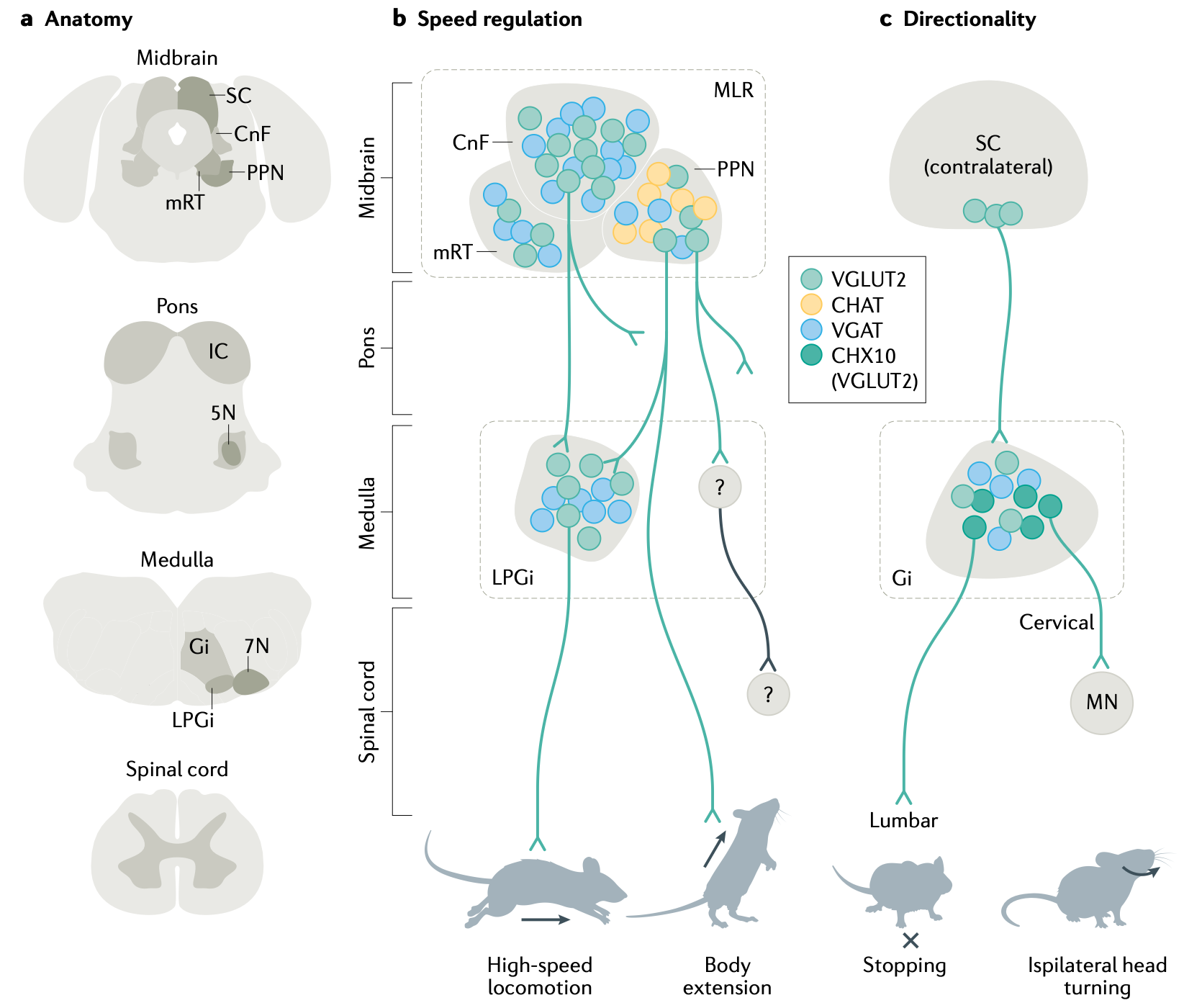
Figure 3: Brainstem levels of control over spinal muscle synergies, across multiple levels from the midbrain to the medulla. MLR = mesencephalic locomotor region; SC = superior colliculus; CnF = cuneform nucleus; PPN = pedunculopontine nucleus; mRT = mesencephalic reticular formation; LPGi = lateral paragigantocellular nucleus; IC = inferior colliculus; 5N = trigeminal motor nucleus; Gi = gigantocellular nucleus; 7N = facial motor nucleus; From Arber & Costa, 2022.

At a broad level, the contributions of each additional level of control are as follows (Grillner & El Manira, 2020; Arber & Costa, 2022; Zaaimi et al., 2018):

• Brainstem nuclei integrate broader sensory inputs to drive more complex, survival-relevant behaviors as combinations of spinal synergies, for example control of locomotor activity (Figure 3) and reaching for food (Esposito et al., 2014; Capelli et al., 2017; Zelenin et al., 2007; Zaaimi et al., 2018).

• The cerebellum performs two different types of predictive learning, which can drive direct tuning of the spinal synergies themselves (Udo et al., 1980; Grillner & El Manira, 2020; Figure 11), as well as the ability to learn different coordinated spatiotemporal patterns across multiple spinal synergies (Berger et al., 2013), with these functions taking place in different pathways through the cerebellum (vestibulospinal, rubrospinal, and reticulospinal).

• The dorsolateral (motor) region of the basal ganglia provides dynamic modulation of ongoing motor actions based on dopamine-driven reinforcement learning mechanisms, to optimize the shaping and selection of actions that lead to reward and avoid negative outcomes (Grillner et al., 2020; Park et al., 2020; Arber & Costa, 2022; Markowitz et al., 2018).

• In mammals, and especially in primates, the frontal neocortex provides more fine-grained spatiotemporal modulation of spinal primitives (Overduin et al., 2015; Aflalo & Graziano, 2006), and even the ability to directly control individual motor units in a way that is otherwise not possible outside of the primate. This is presumably the basis for the ability to develop novel, highly skilled motor programs for tool use in primates and especially humans (Marshall et al., 2022; Strick et al., 2021).

At a more abstract computational level of analysis, the subsumption architecture articulated by Brooks (1986) provides an influential framework for how these stacks of higher-level control might function. Each additional level adds new “higher-order” functionality, while building on top of the existing lower-level functionality. The lower-level systems remain intact, and the system can always fall back on them, but when a higher-level system needs to be engaged, it can selectively inhibit competing lower-level systems in order to take control. The overall behavior is envisioned as an emergent dynamic arising from the parallel interactions between a large number of distributed control systems across different levels.

The PCT framework also envisions a hierarchical system of controllers, but it specifically posits that higher-level control systems function by setting the control parameters of lower-level systems. This is distinct from the inhibition of lower-levels.

Optimal feedback control (OFC) provides a qualitatively different form of control, by positing an optimal online controller mechanism that can use available feedback signals to adaptively control motor parameters. This controller requires an internal forward model, which the cerebellum is widely believed to provide. OFC itself is formulated at an abstract, computational level, so it doesn’t necessarily rest on these neural claims. Nevertheless, the ability of some form of higher-level control to tune spinal-level muscle synergies, and drive other aspects of adaptive control, represents an important distinction between equilibrium-point control and OFC (Shadmehr, 2010).

The UMC (uncontrolled manifold) framework emphasizes the flexibility and adaptability afforded by having entire manifolds of seemingly redundant control parameters (Gelfand & Latash, 1998; Latash et al., 2007), and this flexibility is likely due to the highest levels of control, in the basal ganglia and especially the neocortex, building upon predictive forward models learned in the cerebellum.

These different forms of hierarchical control are not mutually exclusive, consistent with the presence of multiple levels of control, and considerable available evidence. There is however an important contrast to be drawn with more monolithic forms of motor control, such as the notion of a world model controller (see reinforcement learning for further discussion).

In the remaining sections, we cover the basic properties of the skeletal motor system, starting with muscles and moving up the levels of control from there, from the spinal cord to the brainstem, cerebellum, basal ganglia, and neocortex.

Muscles

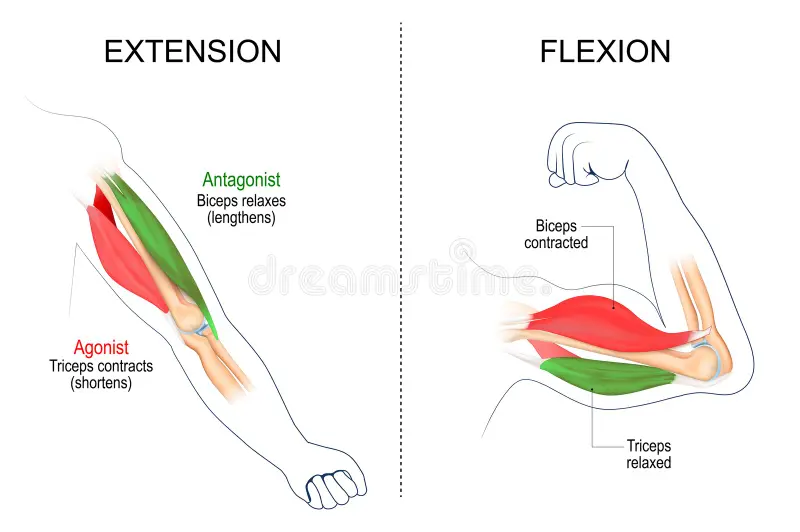
Figure 4: Muscles are organized in opponent pairs, where the contraction of the extensor causes the extension of the limb (e.g., the triceps), while the contraction of the flexor causes the flexion (compaction) of the limb.

Skeletal muscles are organized into opponent pairs (Figure 4), with the contraction of the extensor extending the limb outward (extension), while the contraction of the flexor contracts the limb inward (flexion). Muscles connect to the bones via tendons, which are strong, slightly elastic rope-like tissues made of collagen. Tendons typically wrap around the joints and transmit forces by connecting further down the bone to obtain greater leverage.

Muscles only exert force through contraction, which is driven by the release of acetylcholine from motor neurons, causing actin and myosin fibers to contract. Thus, to actually move a limb, the opponent muscles on each side must be coordinated so that one side contracts and the other side relaxes (which occurs naturally if the muscle is not activated). Furthermore, each overall muscle (e.g., the bicep) is composed of individual motor units that vary in size, each of which has its own motor neuron.

These different motor units are generally activated according to the size principle (Henneman, 1985), where the descending motor control signals first recruit small units, which exert less force, followed by increasingly larger units as the firing rate and number of afferent inputs activated increases (Luca & Erim, 1994). This is because smaller units have a lower threshold, and they also fire at higher rates than larger units. This size principle also optimizes fatigue effects.

The size principle enables a single common-drive unidimensional command input to project to all motor units for a given overall muscle, such that this one input can naturally drive increasing contraction force with increasing neural activity. This is another way in which the motor system reduces the effective dimensionality of the control problem.

Ocular muscles

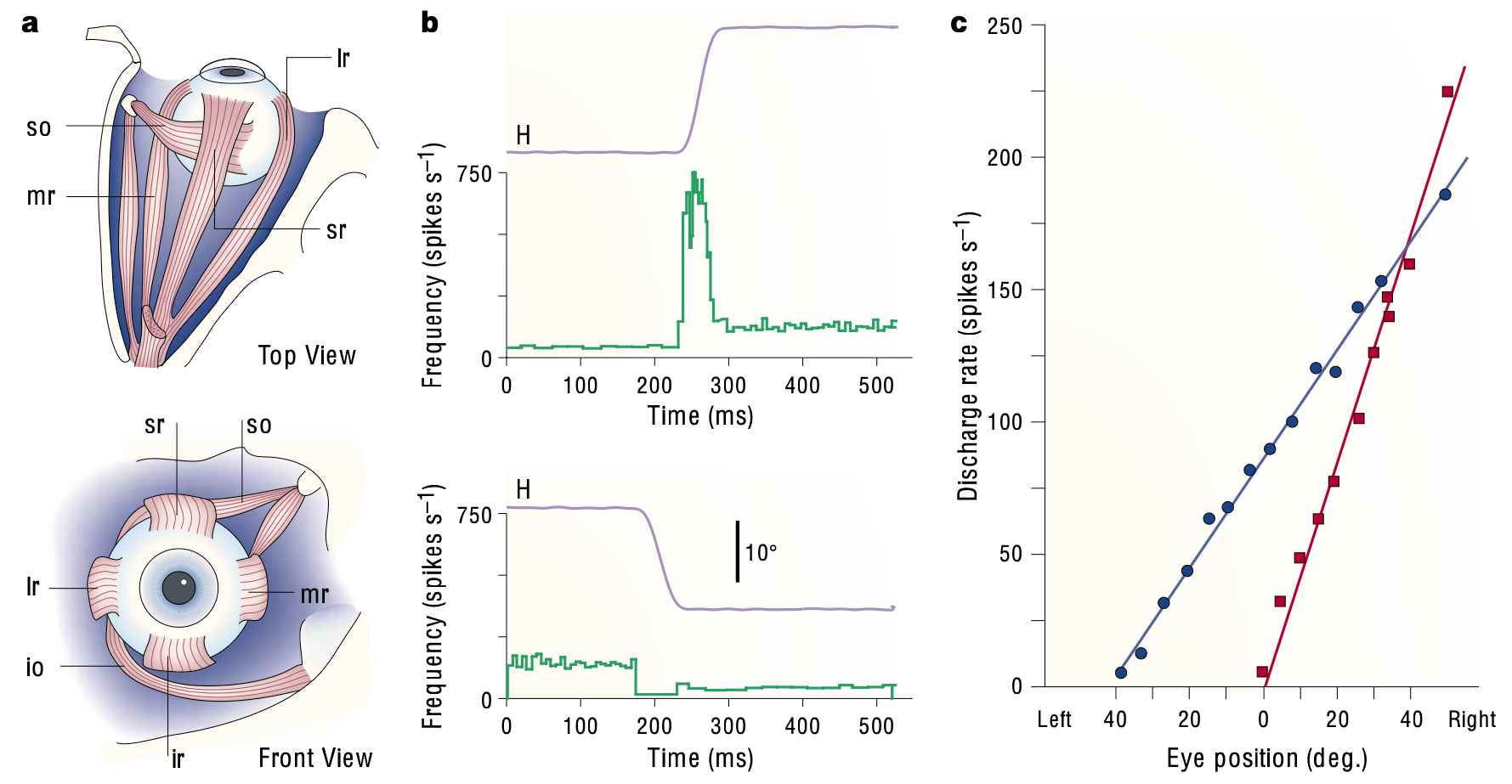
Figure 5: Oculomotor control system. a) Rectus muscles involved in moving the eye, with horizontal motion controlled by the balance between the medial (mr) and lateral (lr) rectus muscles, and vertical controlled by superior (sr) vs. inferior (ir) rectus muscles. b) These muscles are under control of the nucleus abducens (ABN) motor neurons, with a linear relationship between neural firing rate and the position and velocity of the eye, as shown in the plots of H = horizontal eye position above the spike raster plots for a given such neuron. In the top panel, the neuron fires a high-frequency burst to drive a rightward eye movement (right = up in plot), which is ipsilateral to the neuron’s location (right hemisphere, contracting the right-going eye muscles). The subsequent tonic firing rate is linearly related to the subsequent eye position, maintaining the contraction necessary to keep the eye in this off-center location. The bottom panel shows a leftward movement, where the neuron pauses during the movement and then establishes a lower tonic rate of firing. c) The linear relationsip between eye position and firing rate for two different neurons. The difference between ipsilateral – contralateral firing (as an opponent process) provides the most accurate prediction of eye parameters. From Sparks, 2002.

The muscles that control the position of the eyes in a primate have been particularly well studied (Sparks, 2002; Sylvestre & Cullen, 1999; Fuchs et al., 1988), and provide a relatively simple case for motor control, as shown in Figure 5 from Sparks (2002). There is a direct linear relationship between the eye position and eye velocity, and the net firing of the nucleus abducens neurons that control horizontal eye movement. The tonic firing rate of these neurons determines the eye position, as a varying level of muscle contraction is required to keep the eye off of its centered position. A large phasic burst (up to 750 Hz, i.e., a spike every 1.3 ms!) drives the rapid movement of the eye, which is linearly related to eye rotational velocity, with overall burst duration correlating with the duration of eye movement.

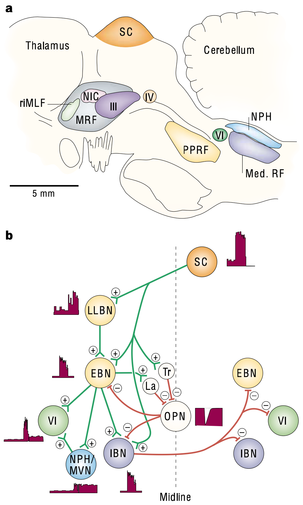
Figure 6: Oculomotor brainstem networks. a) Anatomical organization of areas in a saggital plane of a monkey: MRF = midbrain reticular formation; III = oculomotor nucleus; IV = trochlear nucleus; VI = abducens nucleus; Med RF = medullary reticular formation (saccade generating neurons); NPH = nucleus prepositus hypoglossi (vestibular nucleus); PPRF = paramedian pontine reticular formation (drives horizontal saccades); rlMLF = rostral interstitial nucleus of the medial longitudinal fasciculus (vertical saccades); SC = superior colliculus (optic tectum). b) Network that generates horizontal bursts (BN = burst neuron, located in the PPRF and Med RF): EBN = excitatory burst neuron that directly drives the velocity burst coding of the abducens neurons; IBN = inhibitory; LLBN = long lead (less strongly coupled); MVN = medial vestibular nucleus; OPN = omnipause neuron. Saccades are initiated by trigger (Tr) inputs inhibiting the OPNs, which are then inhibited by latched (La) neurons that are excited by the EBNs during the saccade. From Sparks, 2002.

Figure Figure 6 shows some of the main brainstem areas involved in generating the activity patterns observed in the abducens neurons. The paramedian pontine reticular formation (PPRF) and medulary reticular formation (Med RF) contain various types of bursting and pausing neurons as shown in the figure, which drive the strong phasic bursting associated with saccades (Sparks, 2002). Neurons in the secondary vestibular nuclei (NPH and MVN) drive sustained fixation-maintenance firing in proportion to the current eye position.

These networks are the equivalent of the spinal muscle synergies, but they are located directly in the brainstem due to the eyes being in the head and not the trunk. The particularly simple nature of the eye motor outputs makes this system relatively easy to understand, compared to the more complex, high-dimensional patterns of motor neuron firing required in the locomotor, reaching, and other skeletal muscle domains. Nevertheless, the same kinds of principles presumably apply, in terms of the diversities of neuron firing patterns required to generate the necessary temporal patterns.

The superior colliculus (SC) provides the main input to these brainstem oculomotor areas (Isa et al., 2021). It has a topographic, retinotopic map of neurons that integrate sensory signals from auditory and other modalities, and drive the spatial targeting of visual eye movements (saccades). Consistent with the hierarchical, subsumption nature of motor control, the frontal eye field (FEF) neurons in primary motor cortex typically act through their inputs to the SC to drive more flexible targeting of visual saccades, although they can also drive midbrain circuits directly as well (Sparks, 2002).

Hill-type muscle model

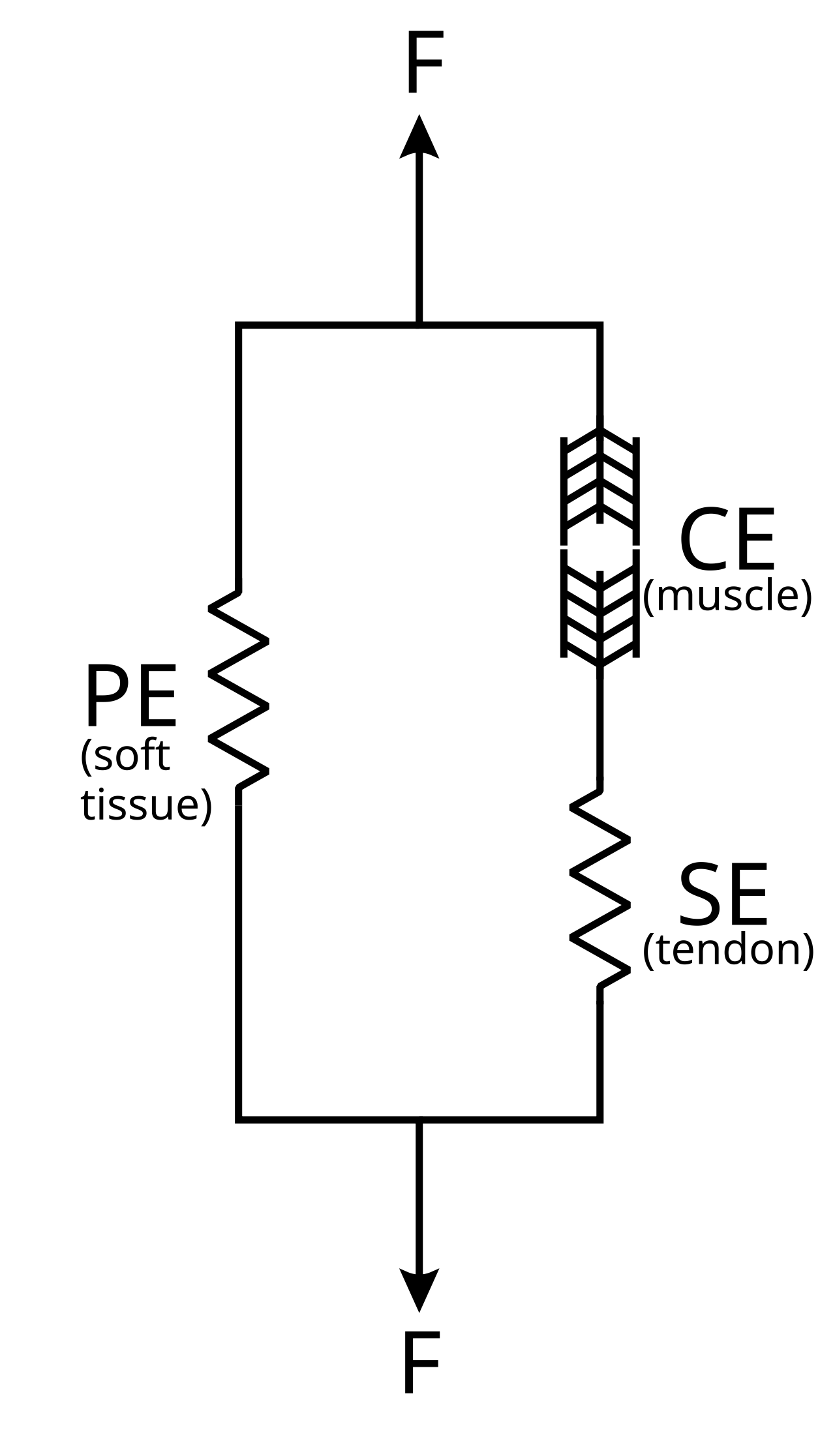
Figure 7: Hill-type muscle model, with a contractile element (CE) representing the muscle itself, a parallel passive element (PE) that represents the spring-like properties of the muscle soft tissue, and a serial spring-like element (SE) representing the tendon. Adapted from Wikimedia Commons.

The standard equations used for simulating muscles are based on the simplified approximation originally developed by Hill (1938), and are thus known as Hill-type muscles (Ritchie & Wilkie, 1958; Zajac, 1989; Millard et al., 2013; see OpenSim for an implementation of the Millard (2013) version: Seth et al., 2018; github). This muscle model has two elements working in parallel (Figure 7): a contractile element (CE) that represents the actual muscle that contracts, and a passive element (PE) that runs parallel to the CE, and represents the spring-like properties of the soft tissue of the muscle. The tendon is represented via a spring-like element in series (SE) with the muscle CE.

Millard et al. (2013) provides a detailed comparison of different variants on this basic muscle model, showing that a damped version of the full model with a spring-like tendon (SE) provides the best compromise between accuracy and computational efficiency. They also analyzed a version with a rigid tendon, which is simpler and faster to compute, but is also significantly more inaccurate.

\[ F_0 (a f_L(l) f_V(v) + f_{PE}(l) + \beta v) cos \alpha - F_0 f_T(l_T) = 0 \]

where \(F_0\) is the peak isometric force, \(a\) is the normalized activation level, \(l\) is the current normalized muscle length, \(v\) is the velocity, \(f_L\) is force-length function, \(f_V\) is the force-velocity function, \(f_{PE}\) is the passive force-length curve, \(\beta\) is the damping factor (.1 default), \(f_T\) is the tendon force-length function, and \(\alpha\) is the pennation angle of the muscle relative to the tendon. These parameters and functions can all be derived anatomically, but do vary for different muscles, so modeling at this level is typically done in a more biologically informed manner.

The equation Eq 1 can be solved for the velocity \(v\) using a derivative-based root-finding method such as Newton’s method, to iteratively update the muscle length in a discrete-time simulation, but this is somewhat computationally intensive.

An alternative solution is to use a piecewise-linear approximation for \(f_V(v)\) (which changes slope significantly at \(v=0\), but is otherwise relatively linear) to allow an analytic solution to solving for \(v\):

\[ v = \frac{f_T(l_T) sec(\alpha) - f_{PE}(l)}{a f_L(l) f_V + \beta} \]

where \(f_V\) represents the relevant slope for the given value of \(v\) (2 iterations are required to converge on that, depending on whether \(v > 0\) or not).

An even simpler and less accurate way to simulate muscles is by manipulating the stiffness and damping parameters on standard physics simulator joints, while updating the joint position values, as we do with the cogent core lab physics models. This requires knowing a target joint position (as in equilibrium-point control), but the stiffness parameter is proportional to the velocity of joint movement, and damping provides the damped spring dynamic.

Spinal cord

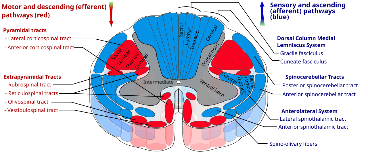
Figure 8: Major pathways in the spinal cord. The ascending sensory pathways originate from neurons in the dorsal horn grey matter (spindle fiber muscle length and golgi tendon stretch proprioception, touch, pain), while the ventral horn contains motor neurons that receive descending motor inputs, and also send ascending efferent copy signals. The intermediate grey matter contains viceral sensory and motor neurons, and throughout there are interneurons that are actually the primary targets of most of the descending control inputs. Adapted from Wikimedia Commons.

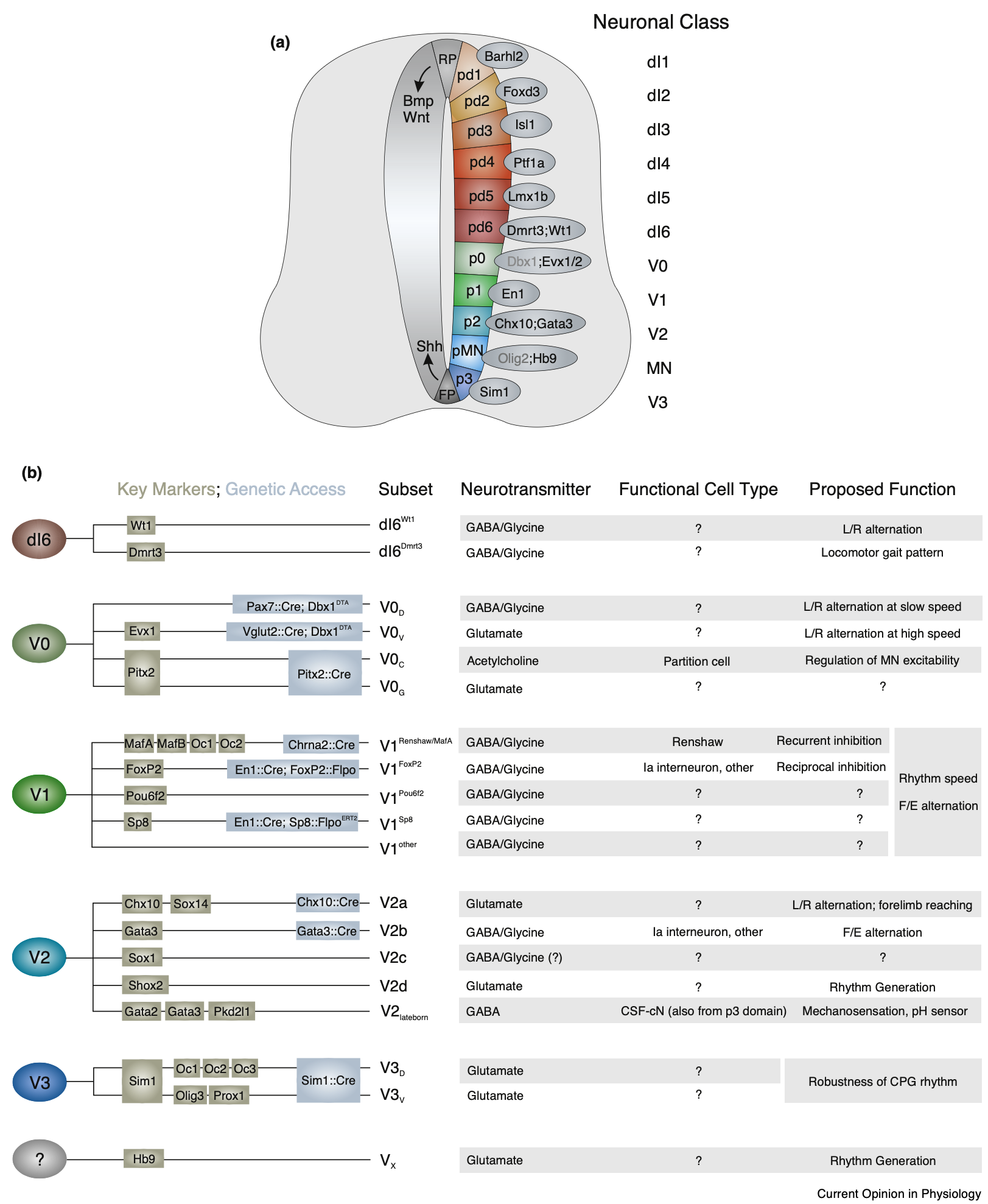
Figure 9: Identified categories of spinal interneurons, organized according to dorsal vs. ventral location, and ordered by date of birth. Double-click for a larger version. From Bikoff, 2019.

The spinal cord is far from a passive motor output system, as discussed above with respect to the muscle synergies that are implemented at the lowest level directly by the extensive neural networks of the spinal cord. These neural networks involve primary sensory and motor neurons and many different subtypes of interneurons with different patterns of connectivity and neurotransmitters (Figure 9 from Bikoff, 2019; see also Sengupta & Bagnall, 2023).

The inputs and outputs of this system are organized into different tracts of long-range axonal fibers as shown in Figure 8 (see also Tan et al., 2023; Watson & Kayalioglu, 2009), with the dorsal horn grey matter having the cell bodies of sensory neurons that respond to a range of somatic inputs, which are conveyed through the ascending pathways up into many areas of the brain, including finally the thalamus and somatosensory neocortex. These somatosensory signals include:

• • Touch, vibration, pressure, and tension signals from mechanoreceptors in the skin and subcutaneous areas.
• • Pain and temperature from nociception receptors.
• • Proprioception signals via muscle spindle fibers that respond to changes in the length of a muscle (via type Ia sensory neurons) and overall muscle length (type II neurons), and Golgi tendon receptors that respond to the stretch or load on a limb (type Ib neurons).

The ventral horn grey matter contains primary motor neurons that directly drive contraction of muscles, while the intermediate grey matter area (at certain levels of the spinal cord) contains sensory and motor viceral neurons.

The extensive networks of interneurons directly receive descending motor command inputs and local (and more distal) sensory inputs, to implement the muscle synergies that produce the low-dimensional vocabulary of motor actions. The direct incorporation of the sensory signals (especially the muscle spindle length signals) allows these muscle synergy components to be robust and adaptive, simplifying the job of the descending motor control inputs.

Whereas these interneurons were previously categorized into a few specific classes (McCrea, 1992; Hultborn, 2006; Côté et al., 2018), a more modern strategy based on developmental neuron birth order and genetic labeling has allowed a more reliable understanding of the complex nature of these spinal networks, as shown in Figure 9 (Bikoff, 2019; Sengupta & Bagnall, 2023). Critically, sensory inputs project to multiple different such interneurons, and each interneuron can receive multiple different types of inputs, so unlike the historical accounts, everything is much more complex and difficult to categorize (Jankowska, 2022; Côté et al., 2018).

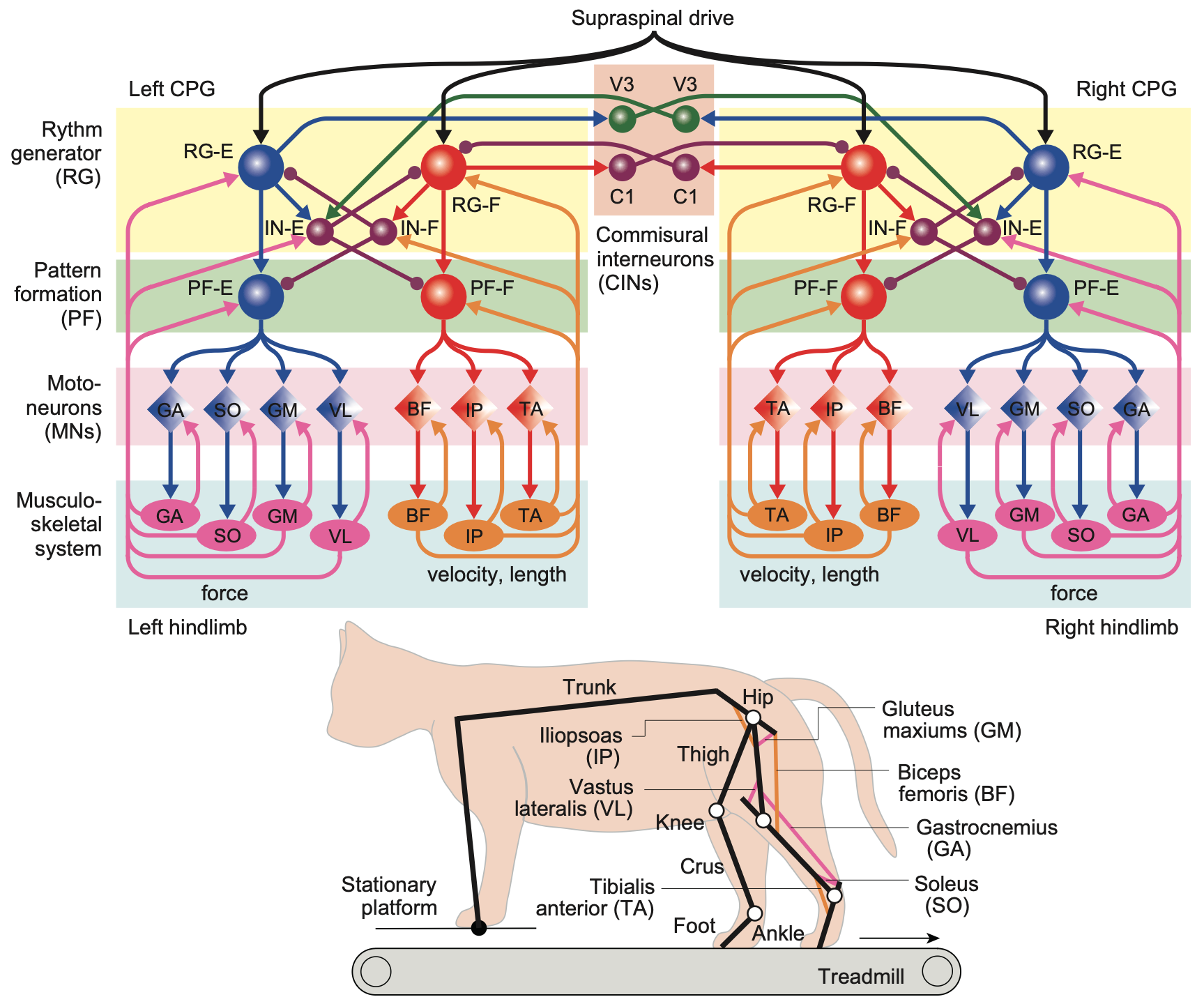
Figure 10: Detailed circuit-based model of spinal central pattern generator (CPG) circuitry that can accurately simulate many aspects of hind-limb locomotion in the spinal cat. The interneurons are labeled functionally, with the suffix -E for extensor and -F for flexor: RG = rhythm generating; PF = pattern formation; IN = inhibitory interneurons. The velocity, length neurons in orange are the proprioceptive (spindle fiber) neurons that provide critical sensory feedback into the motor neurons (restricted to flexors) and there is also critical efferent copy feedback from force-generating motor neurons. Note that the descending supraspinal drive inputs go into the top-level RG interneurons, not the motorneurons. From Shinohara et al., 2025.

A recent example of the sophistication and complexity of these spinal circuits is shown in Figure 10 from Shinohara et al. (2025) (see Danner et al., 2017 for a review of related models and Aoi et al., 2019 for a human bipedal example), which can simulate many aspects of hindlimb locomotion behavior, including when the foot lands in a “hole” where there is no support. This robust adaptive behavior results from the direct incorporation of proprioceptive length and velocity signals from muscle spindle fibers, along with cutaneous touch inputs, into the overall circuit. The connectivity was optimized to minimize overall energy consumption and to adapt to uneven surfaces, and then automatically generalized from there to this lack-of-support situation.

Critically, these robust adaptive behaviors require bilateral coordination across hemispheres, because if one foot goes unsupported, the load must be taken up by the other foot, until a secure footing is obtained. This model can predict detailed patterns of movement and neural firing signals in corresponding experimental preparations, providing strongly validated understanding of how these circuits function.

Interestingly, these circuits also have the property that they modulate the speed of locomotion as a function of the firing rate of descending input control signals, making the job of the higher brain areas much simpler compared to the prospect of having to learn how to perform all of this complex coordinated motor behavior.

A more abstract analytic approach to understanding these CPG dynamics used state-space methods to characterize the dynamics across the entire population of spinal interneurons involved in locomotion (Wimalasena et al., 2025). This approach forgoes the ability to account for the detailed behavior of individual identified interneurons, but allows the full population dynamics to be incorporated.

Primates and humans have more control

There is considerable evidence that primates, and especially humans, have a much greater ability to directly control individual muscles, beyond what is exposed by the muscle synergies and CPG circuits implemented by the spinal cord and brainstem networks (Grillner & El Manira, 2020; Grillner, 1981). For example, Marshall et al. (2022) showed evidence of more flexible recruitment of motor units that goes beyond the rigid constraints of the size principle as discussed above. There are also a larger number of secondary motor areas in primates that have more focal, specialized projections to specific limbs (Strick et al., 2021).

Interestingly, despite the idea that the extra degrees of freedom associated with this increased level of fine-grained control, there is a reliable relationship between brain size and age of first locomotion that humans and other primates still obey (Garwicz et al., 2009).

The development of motor control in humans was hypothesized by Bernstein (1996) to follow a trajectory from relying on more rigid, evolutionarily encoded motor programs, to gradually allowing more flexible, higher-dimensional control from the neocortex to be learned. Evidence is consistent with this hypothesis (Hinnekens et al., 2023; Dominici et al., 2011).

Higher level systems

In the remaining sections, we explore in more depth some of the issues associated with the neural systems that provide higher levels of control. See Bizzi & Ajemian (2020) for a recent broad commentary on these systems.

Cerebellum

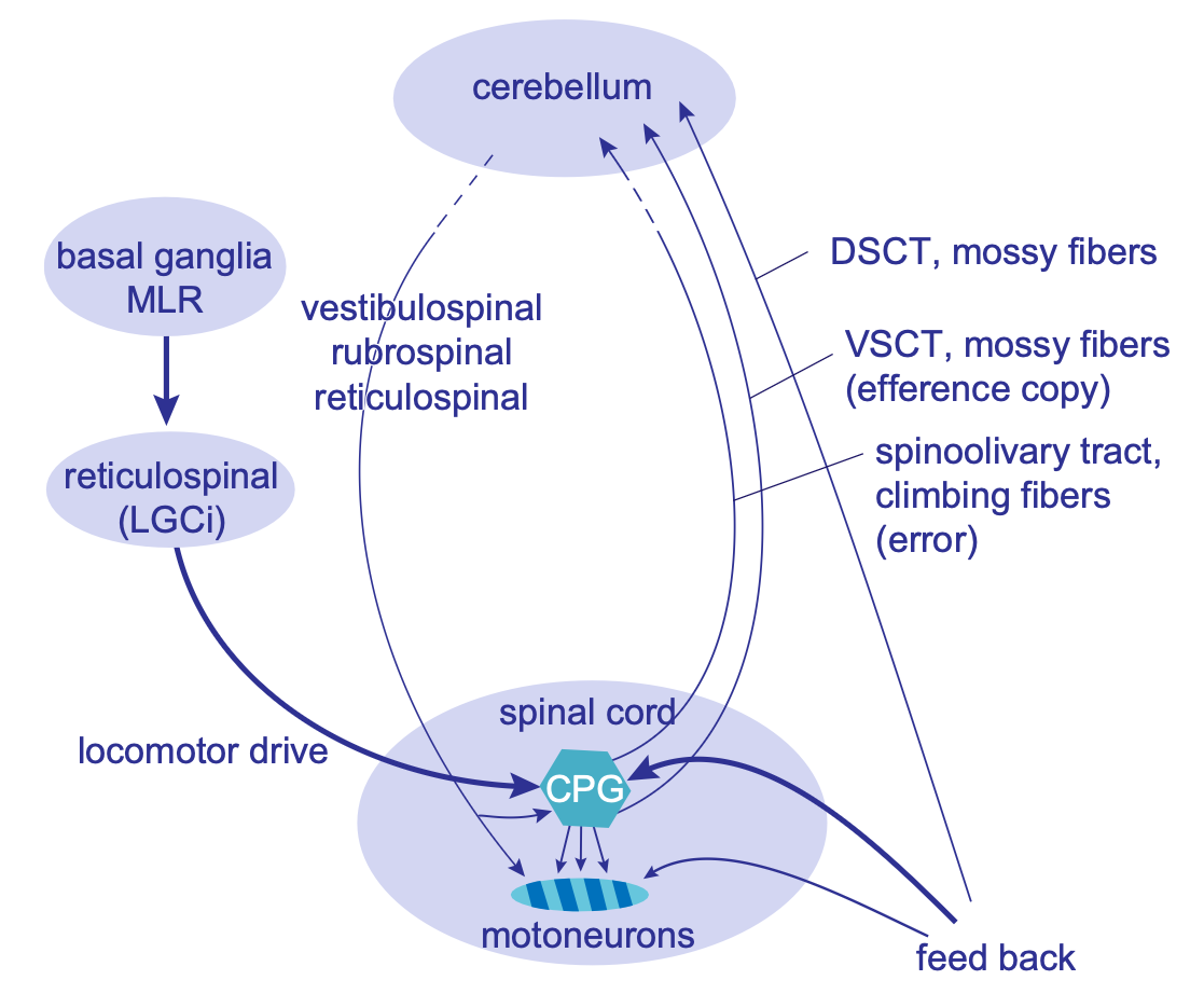
Figure 11: Pathways by which the cerebellum can control the tuning of spinal muscle synergies (CPGs: central pattern generators). DSCT = dorsal spinocerebellar tract; VSCT = ventral spinocerebellar tract; MLR = mesencephalic locomotor region; LGCI = lateral paragigantocellular nucleus. From Grillner & El Manira, 2020.

The cerebellum learns by predicting specific sensory signals using a broad range of other ongoing sensorimotor signals. It can uses this predictive learning to adaptively filter expected signals, and also provide earlier active predictions of these signals, as a forward model. These learning abilities can be used to drive the fine tuning of the spinal CPGs / muscle synergies, as shown in Figure 11 from Grillner & El Manira (2020).

The cerebellum can also use predictive learning to activate muscle synergies and other higher-level motor programs, to accomplish more well-coordinated motor actions. One well-studied example is in the case of the vestibulo-ocular reflex (VOR), where the anticipated effects of head rotation can drive anticipatory, compensatory eye movements in the opposite direction, to maintain a stable visual percept.

However, some times the goal is instead to generate a saccade to fixate on a particular point in space, using a combination of head and eye movements. In this case, the VOR reflex must be inhibited, and a different saccadic eye movement programmed, which takes into account the anticipated head movement so that the two actions together end up with the eyes fixating on the target location. Thus, this flexible action space of VOR vs saccades represents a good well-studied example of how higher-level control works in the cerebellum.

It is important to understand that the cerebellum manages a set of control “knobs” for different motor programs, but it does not itself decide what to do with these knobs. That is the job of the basal ganglia, which has the relevant reward-based learning mechanisms to make such decisions. The cerebellum learning is instead optimized for smooth coordination across different programs, by leveraging its ability to anticipate the effects of motor actions, and drive everything according to these predictions.

Basal ganglia

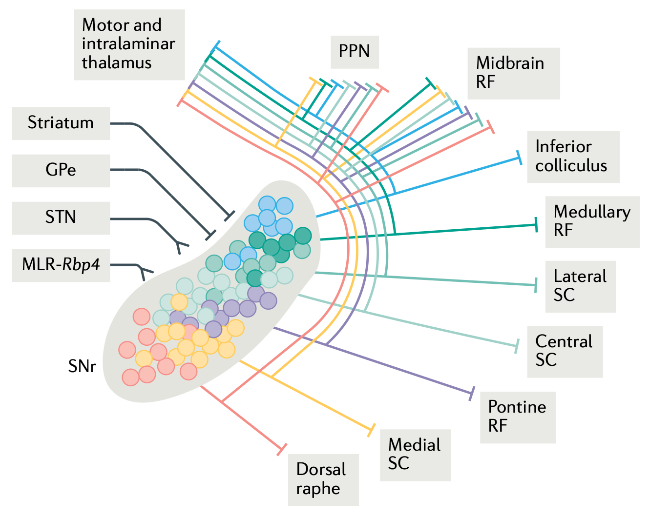
Figure 12: Motor output pathways of the basal ganglia, via the SNr (substantia nigra pars reticulata). These extensive outputs allow the basal ganglia to sculpt appropriate sequences of muscle synergy programs in these areas, using powerful dopamine-based reinforcement learning mechanisms. From Arber & Costa, 2022.

The dorsolateral (DL) basal ganglia (BG) drives learning of a broad range of output neurons (in the SNr and GPi) that project down into all of the relevant lower-level motor control areas (Figure 12, from Arber & Costa, 2022). As discussed in Motor activity in DL, the BG provides dynamic, continuous modulation of descending motor signals, which enables powerful gradient-based search to drive learning, which is much more efficient than any form of discrete Go vs. NoGo motor selection logic.

The BG also sends ascending input into the frontal cortex, via various thalamic pathways, but the diffuse nature of these pathways (relative to the much more specialized and focal output from the SNr as shown in Figure 12) makes it unclear what the functions of these ascending signals are. We discuss some possibilities in the next section.

Frontal cortex

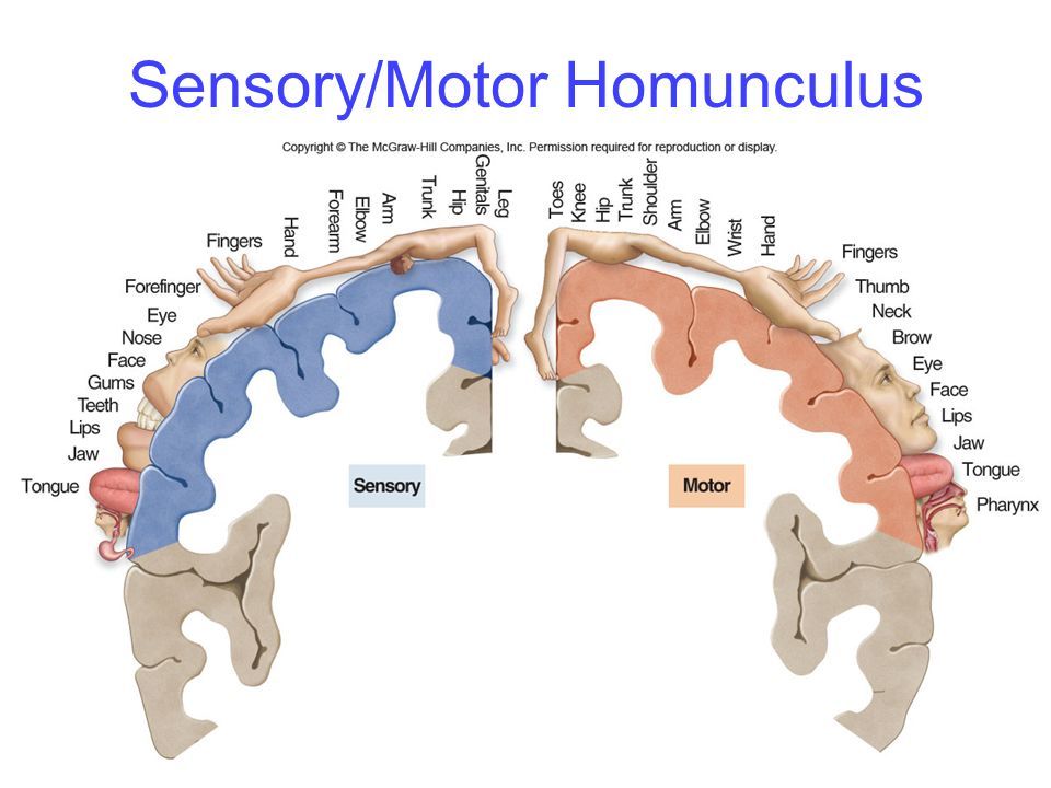
Figure 13: The homunculus (“little person”) organization of the primary sensory (S1) and primary motor (M1) cortical areas, which sit across the central sulcus from each other, and are densely interconnected. S1 provides strong driver inputs to M1, both directly via corticocortical pathways, and indirectly via projections going through the posterior medial nucleus of the thalamus (POm).

The neocortex is the highest level of motor control (in mammals), with an extensive mapping of all motor and somatosensory signals organized in a somatotopic map that is described as a kind of homunculus (“little person”) inside the brain (Figure 13). Consistent with the increasing importance of the neocortex in primates and especially humans, the large amount of neural tissue devoted to these somatosensory and motor representations enables people to exhibit the most flexible and varied forms of motor behavior, for example everything on display at the Olympics every couple of years.

Unlike most of the rest of the brain, the neocortex is thought to gain almost all of its functionality through learning taking place during an animal’s lifetime. This poses an important challenge for the motor system: how can the motor cortical areas learn to “speak the language” of the spinal cord, to provide meaningful motor control signals?

Our hypothesis is that the same mechanisms used in predictive learning of sensory and other representations in the cortex, supported by the pulvinar and MD nuclei in the thalamus, could also be at work on the motor side in frontal cortex areas. As discussed in frontal thalamus, area VL (ventrolateral) receives driver inputs from the cerebellar nuclei, and sends more focal core-like inputs into the middle layers of motor cortex. These inputs should be sufficiently specific to drive the learning of appropriate motor commands reflecting the temporal difference between the original command over the motor cortex, and the subsequent efferent copy reflecting what the motor system actually did with the command.

There are natural delays between the time when the frontal cortex drives a descending motor command and the time when the efferent copy signals from these ascending pathways reflect the actual low-level motor commands that were actually generated (with significant contributions and shaping by all of the above areas). This delay provides the temporal derivative dynamics needed to drive predictive learning, where the motor cortex is effectively learning to predict what the motor system will do in response to the commands it sends down. This hypothesis is consistent with the “big loop” of descending and ascending motor signals shown in Figure 14 (from Arber & Costa, 2022).

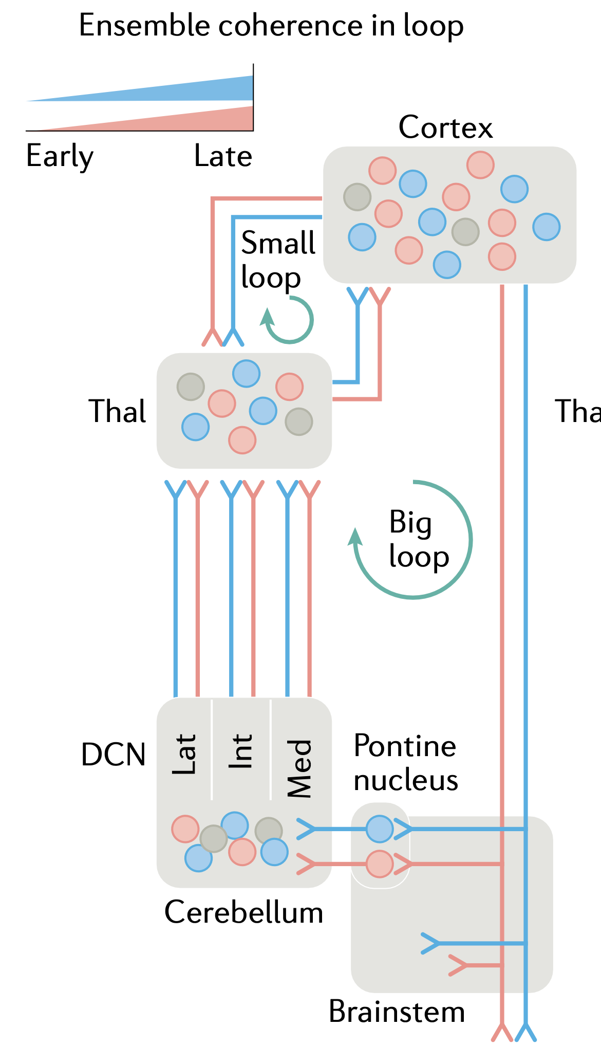
Figure 14: The “big loop” of motor processing, which could support a form of predictive learning to train frontal cortex. The thalamus (VL = ventrolateral specifically) receives strong driver inputs from the DCN (deep cerebellar nuclei), and standard non-driver inputs from motor cortex, and projects focal (“core-like”) inputs into motor cortex, that would be capable of providing specific motor training signals. The difference over time between these two inputs can drive the temporal derivative error-driven learning mechanism. The small loop involves distinct areas of thalamus (VA, VM) with broad (“matrix-like”) connectivity that would not likely provide useful specific training signals. Instead, it may be important for driving the transition from preparatory to driving motor activity states in cortex. From Arber & Costa, 2022.

Furthermore, there are important driver-like pathways from the somatosensory cortex (S1) to motor cortex (M1), both directly via corticocortical pathways (Petrof et al., 2015) and through thalamic pathways via the posterior medial thalamus (POm) (Mo & Sherman, 2019). Given that S1 also receives extensive ongoing inputs reflecting the sensory consequences of motor actions, including efferent copy signals, and all of the proprioceptive signals involved in providing feedback control over spinal and brainstem motor synergies, this provides the opportunity for cortex to both leverage such signals for online feedback control itself, and to use these signals for driving learning of motor representations as well, via the same kind of predictive learning mechanisms that obtain in the VL-based big-loop pathway.

The role of these somatosensory signals in training motor learning in the neocortex via predictive learning is thus isomorphic with the way the cerebellum learns via predictive learning of sensory outcome signals. Whereas the cerebellum is organized to be able to provide online modulation of ongoing motor actions at a fine-grained timescale, the neocortex generally operates at slower timescales and is more important for using its bidirectional connectivity and constraint satisfaction processing to select and shape actions.

The “small loop” in Figure 14 involves different thalamic neurons and areas, specifically ventral-anterior and medial (VA, VM), which are matrix-like and send broad, diffuse connectivity to the most superficial layer of motor cortex. Thus, these areas are not suitable for driving learning (and do not get excitatory driver inputs), but they may play a critical role in driving the transition from a preparatory state of activity to the activity patterns that actually drive motor activity (Economo et al., 2018; Guo et al., 2018; see systems-level dynamics in the prefrontal cortex page for more discussion).

More abstract state-space analyses of motor activity have consistently shown that preparatory motor activity lives in a null space relative to the activity states that actually drive lower-level motor output pathways (Churchland & Shenoy, 2024). These output pathways are driven by layer 5b PT (pyramidal tract) neurons (specifically in the lower 5b; Economo et al., 2018), which are selectively targeted (in their apical tufts) by the broadly projecting matrix-like pathways from the VA thalamic areas that receive disinhibitory basal ganglia inputs (see frontal thalamus). Therefore, although it is not as simple as the exclusive activity of these PT neurons by BG inputs, it is likely that the transition from the preparatory null space to the motor output space is facilitated by these BG signals.

There are many studies on the nature of motor cortical representations in relation to final motor output parameters. All manner of relevant signals have been decoded from individual neurons, but as usual, the overall distributed representations are more relevant (Georgopoulos & Carpenter, 2015). Aflalo & Graziano (2006) showed that final hand posture accounts for most of the variance, consistent with the general nature of muscle synergies as discussed above. However, other factors such as speed, curvature of space, distance and force were also coded.

Another study explored cases where more complex sequences of motor actions were required, and showed that a temporal sequence of postural configurations is specified (i.e., a spatiotemporal synergy; Overduin et al., 2015).

At a more abstract level of analysis, Meyer et al. (1982) synthesized extensive psychophysical literature on speed and accuracy of motor movements in humans, to develop a symmetric impulse control model that specifies the force and duration parameters as curves with an initial acceleration phase for the first half, followed by a symmetric deceleration phase in the second half. Both the force and time parameters of these curves can be controlled by people. There is evidence that ballistic movements are made below around 260 ms, with multiple iterations of visually corrected movement updates happening after that, time permitting (see also Meyer et al., 1990).