
Hebbian learning
The famous Canadian psychologist Donald O. Hebb predicted the nature of the NMDA channel many years in advance of its discovery, just by thinking about how learning should work at a functional level. Here is a key quote (Hebb, 1949):
Let us assume that the persistence or repetition of a reverberatory activity (or “trace”) tends to induce lasting cellular changes that add to its stability.… When an axon of cell A is near enough to excite a cell B and repeatedly or persistently takes part in firing it, some growth process or metabolic change takes place in one or both cells such that A’s efficiency, as one of the cells firing B, is increased.
This can be more concisely summarized as cells that fire together, wire together. As discussed in detail in synaptic plasticity, the NMDA channel is essential for this process, because it requires both pre and postsynaptic activity to allow \(Ca^{++}\) to enter and drive learning. It can detect the coincidence of neural firing. Interestingly, Hebb is reputed to have said something to the effect of “big deal, I knew it had to be that way already” when someone told him that his learning principle had been discovered in the form of the NMDA receptor.
Mathematically, we can summarize Hebbian learning as:
\[ \Delta w \propto x y \]
where \(\Delta w\) is the change in synaptic weight w, as a function of sending activity x and receiving activity y. If you only use this equation, and the activity values are biologically realistic firing rates, which are only positive numbers, then the synaptic weight can only go up in value. Thus, some additional factors are required in this case to produce a more balanced pattern of weight increases (LTP) and decreases (LTD). A few such factors are reviewed below.
However, even with a well-balanced form of Hebbian learning, and including the widely investigated spike timing dependent plasticity (STDP; Bi & Poo, 1998) variant of Hebbian learning, the primary issue is that there is no mathematical or computational basis to expect that it will actually enable a network of neurons to learn the kinds of cognitive and behavioral functionality that humans and other animals exhibit. It is simply a “heuristic” principle that might make some intuitive sense, but all of the available evidence strongly indicates that it lacks the general purpose flexibility of error-driven learning mechanisms. See the pattern associator simulation and hidden layer simulation for simple examples demonstrating this difference between Hebbian and error-driven learning.
The difference between Hebbian learning and error-driven learning at a mathematical level comes down to the presence of some kind of difference-based element in equation, that drives learning based on a contrast between two factors, rather than just the “main effect” of raw association. For example, the GeneRec version of error-backpropagation learning results in the Contrastive Hebbian Learning (CHL) equation, which was originally developed in the Boltzmann machine (see also Movellan & McClelland, 1993):
\[ \Delta w \propto (x^+ y^+) - (x^- y^-) \]
You can see that this is just a difference between two Hebbian factors as in Eq 1, where the + superscript indicates neural activity in the plus phase when the correct answer is present, while the - indicates the minus phase where the network is generating its own answer, based on the existing synaptic weights in the network. In the context of predictive learning, the minus phase immediately precedes the plus phase, as the prediction of what is going to happen, followed by what actually does happen.
This CHL equation provides a useful qualitative summary of the actual kinase algorithm equations used in Axon, and illustrates how the intuitive core of Hebbian associative learning and the pre-post contingency of the NMDA receptor can all be carried over into the much more computationally powerful error-driven learning domain.
Furthermore, a central premise of the Leabra algorithm is that a very small amount of Hebbian learning can be combined with this CHL-based error-driven learning, where the Hebbian factor acts as a kind of bias or regularization factor that shapes the learning toward encoding statistical regularities (see bias-variance tradeoff for general principles). This is similar to weight decay which is used in abstract neural network models and in statistical regression, except with Hebbian learning you also have weight values going up and not just decaying toward zero.
Interestingly, the inherent noise present in the Axon discrete spiking dynamics produces many of the same effects as the additional Hebbian component added to Leabra, and we found that it was therefore unnecessary (and not beneficial) to add a Hebbian component in addition to the primary error-driven learning.
One hypothesis that remains to be explored in implemented Axon models, is that layer 4 of the neocortex, which receives the bottom-up sensory inputs from the thalamus in primary sensory areas, performs a primarily Hebbian form of “pre processing” of these sensory inputs. Layer 4 has a different class of excitatory neurons, stellate cells (vs the predominant pyramidal neurons in the other layers), which have much more localized patterns of connectivity, and largely have feedforward outputs to the superficial layers 2⁄3. All of these features are suggestive of a localized stage of processing that performs some form of useful transformation on the incoming signals. See the V1 self organizing simulation for an example of this form of processing applied to primary visual cortex (V1) sensory inputs.
In the remainder of this page, various standard forms of Hebbian learning are reviewed, providing a basis for understanding what this type of learning can accomplish.
Self organization with inhibitory competition
There are a number of self organizing models that combine Hebbian learning with various forms of inhibition among neurons within a hidden layer. The inhibitory competition forces individual neurons to specialize on encoding different separable features of the input environment, instead of having every neuron learning the same thing. Metaphorically, inhibition is like evolutionary survival-of-the-fittest: the neurons that respond the best to a given set of input stimuli win the competition to represent such inputs, and thus end up further specializing their encoding on that subset of the overall space.
At an abstract mathematical level, the principal components analysis (PCA) method provides a good example of what these algorithms can accomplish, by developing new more efficient and systematic ways of encoding the most important components latent in the inputs. PCA extracts correlations among the input signals, and shows how Hebbian learning is likewise driven to learn the correlational structure of its inputs.
Some of the earliest models of this type were developed by Teuvo Kohonen and colleagues (Kohonen, 1977; Kohonen, 1998; Kohonen & Hari, 1999). In these self organizing map (SOM) models, iterative Hebbian-like learning and a simple form of inhibitory competition produces a topographic mapping of the features in the input space, organized across the 2D geometry of the hidden layer. This kind of topographic mapping is well-established in primary sensory areas of the neocortex. For example, primary visual cortex (V1) has a topographic organization of neurons encoding different orientation angles of edge detectors (see V1 self organizing simulation), as originally discovered by Hubel & Wiesel, 1962 in their Nobel-prize winning research.
The SOM model implements inhibitory competition by selecting the individual neuron that received the greatest amount of “excitation” from the current input, which is typically computed in terms of the minimum distance between the synaptic weights and the input activity vector, rather than the dot product. This neuron is then used as the center point of a gaussian-shaped “bump” of activity that defines the amount of learning each neuron experiences, falling off as a function of the 2D distance from the central best-matching neuron. The following Hebbian learning equation is used:
\[ \Delta w_{ij} \propto y_j (x_i - w_{ij}) \]
where \(y_j\) is the gaussian-shaped bump activity for receiving neuron \(j\), \(x_i\) is the activity of input neuron \(i\), and \(w_{ij}\) is the synaptic weight between the two neurons.
This learning rule moves the synaptic weight to match the input activity pattern, instead of simply increasing weights among co-active neurons. Thus, it will drive increases and decreases (LTP and LTD) based on those differences. Nevertheless, it is still Hebbian in nature, in that it is purely driven by the input activity and does not include an error signal. We will see related forms of learning in the algorithms explored below. See the wikipedia SOM page for more details.
The competitive learning model of Rumelhart & Zipser (1985) and subsequent soft competitive learning models (Nowlan, 1990; Nowlan & Hinton, 1993) are similar to the SOM in that they drive learning via a strong competition among receiving neurons, but they forgo the 2D topography imposed by the gaussian bump of activity, and thus learn more arbitrary, high-dimensional representations. See self organizing simulation for an example of how these types of models can extract the correlational structure of a simple environment composed of line elements.
The models of Bednar & Miikkulainen (2003) and Bednar (2012) provide a more biologically detailed model of this self-organizing learning process as applied to primary visual cortex (see V1 self organizing simulation for a related model).
BCM
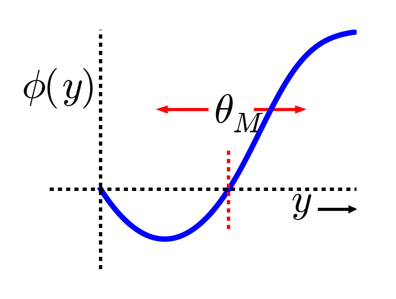
Figure 1: The BCM learning function, which is consistent with the empirical relationship between intracellular Ca++ and sign of synaptic plasticity changes: LTD for elevated but moderate, and LTP above a higher threshold. In BCM, the threshold between LTD and LTP changes as a function of the receiving neuron activity y, producing a homeostatic (negative feedback) dynamic that keeps activity within reasonable ranges.
The BCM (Bienenstock et al., 1982) version of Hebbian self-organizing learning uses a different approach to accomplish a similar effect as direct inhibitory competition. Specifically, it uses a homeostatic mechanism that keeps each receiving neuron at a consistent average level of activity, by using a dynamic floating threshold that shifts the balance between weight decreases (LTD) and weight increases (LTP) as a function of receiving neuron average activity (figure_bcm]). When a neuron’s activity is relatively high, then there is more LTD than LTP, thus driving the activity downward, and vice-versa for lower levels of activity.
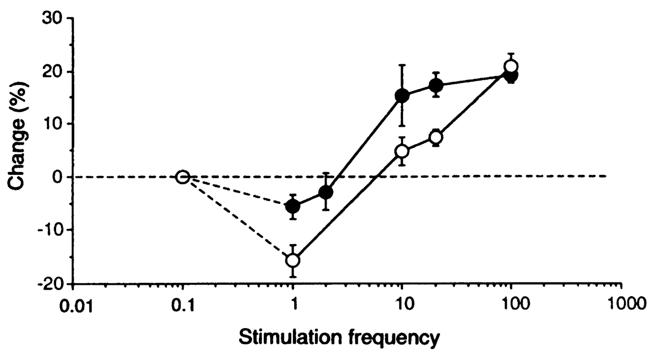
Figure 2: Synaptic plasticity data from dark reared (filled circles) and normally reared (open circles) rats, showing that dark reared rats appear to have a lower threshold for LTP, consistent with the BCM floating threshold. Neurons in these animals are presumably much less active overall, and thus their threshold moves down, making them more likely to exhibit LTP relative to LTD. Reproduced from Kirkwood, Rioult, & Bear (1996).
When seeded with random initial weights, this homeostatic mechanism causes individual neurons to specialize on specific subsets of the input space, just as the direct inhibitory competition does in the above algorithms. It is clear that direct pooled inhibition plays a major role in shaping activity in the neocortex, but there is also evidence for homeostatic-like mechanisms as well. For example, Figure 2 shows that the relative threshold for LTP vs LTD does shift as a function of overall activity (Kirkwood et al., 1996).
In the Axon algorithm, we use a version of the sleep-based synaptic reorganization mechanism described by Torrado Pacheco et al. (2021), which rescales synaptic weights learned during the day according to individualized target average activation levels for each neuron (see Slow weights). This has homeostatic properties similar to the BCM algorithm, and is critical for preventing individual neurons from “hogging” the representational space. The Leabra algorithm uses a version of the BCM algorithm to accomplish this function, and to drive the regularizing effects of Hebbian learning.
Hebbian learns correlations
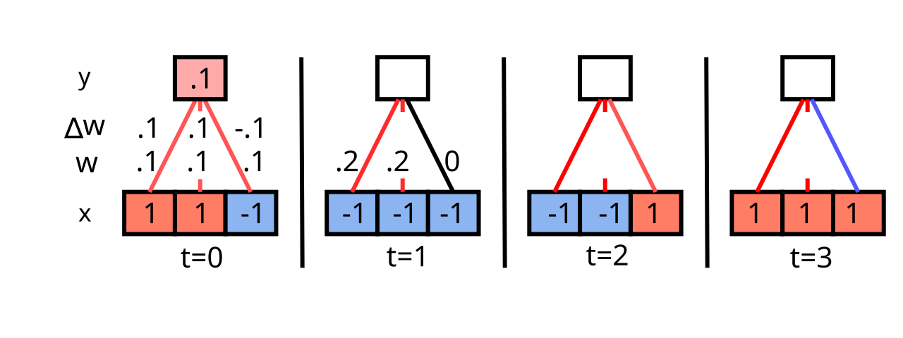
Figure 3: Simple Hebbian learning demonstration across 4 time steps (t=0 thru 3). The bottom row has 3 input units, the last of which fires in an “uncorrelated” fashion with the other two. They all start out with weights w = .1. Receiving activity is just a linear sum of the sending activations times weights: y = \sum x w = .1 for the first time step. Learning is simple Hebbian: \Delta w = xy. As you fill in the remainder of the activations, weights, and weight changes, you will find that the two correlated input units dominate the receiving unit activation, and thus they end up being correlated in their activity, causing their weights to always increase. The third unit sometimes goes up and sometimes down, with no net increase over time. Thus, Hebbian learning discovers correlations in the inputs.
Figure 3 shows a simple demonstration of how Hebbian learning causes the receiving network to discover correlations in the patterns of input unit activation. The input units that are correlated end up dominating the receiving unit activity, and thus the receiving unit ends up being correlated with this subset of correlated inputs, and their weights always increase under the Hebbian learning function. Uncorrelated inputs bounce around without a systematic trend. If you keep going, you’ll see that the weights grow quickly without bound, so this is not a practical learning function, but it illustrates the essence of Hebbian learning.
Next, we do some math to show that the simplest version of Hebbian correlational learning, in the case of a single linear receiving unit that receives input from a set of input units, result in the unit extracting the first principle component of correlation in the patterns of activity over the input units.
Because it is linear, the receiving unit’s activation function is just the weighted sum of its inputs, i.e., the dot product (see linear algebra):
\[ y_j = \sum_k x_i w_{ij} \]
(all of the variables are implicitly a function of the current time step \(t\) reflecting different inputs). The weight change is:
\[ \Delta_t w_{ij} = \epsilon x_i y_j \]
where \(\epsilon\) is the learning rate and \(i\) is the index of a particular input unit, and weights just increment these changes over time:
\[ w_{ij}(t+1) = w_{ij}(t) + \Delta_t w_{ij} \]
To understand the aggregate effects of learning over many patterns, we can just sum the changes over time:
\[ \Delta w_{ij} = \epsilon \sum_t x_i(t) y_j(t) \]
If you set \(\epsilon = 1 / N\), where \(N\) is the total number of patterns in the input, then the sum turns into an average:
\[ \Delta w_{ij} = \langle x_i y_j \rangle_t \]
Next, substitute into this equation the formula for \(y_j\) (using \(k\) now for the input index), showing that the weight changes are a function of the correlations between the input units:
\[ \Delta w_{ij} = \langle x_i \left(\sum_k x_k w_{kj} \right) \rangle_t \]
\[ = \sum_k \langle x_i x_k \rangle_t \langle w_{kj} \rangle_t \]
\[ = \sum_k \bf{C}_{ik} \langle w_{kj} \rangle_t \]
This new variable \(\bf{C}_{ik}\) is an element of the correlation matrix between the two input units \(i\) and \(k\), where correlation is defined here as the expected value (average) of the product of their activity values over time (\(\bf{C}_{ik} = \langle x_i x_k \rangle_t\)). You might be familiar with the more standard correlation measure:
\[ \bf{C}_{ik} = \frac{\langle (x_i - \mu_i)(x_k - \mu_k) \rangle_t} {\sqrt{\sigma^2_i \sigma^2_k}} \]
which subtracts away the mean values (\(\mu\)) of the variables before taking their product, and normalizes the result by their variances (\(\sigma^2\)). Thus, an important simplification in this form of Hebbian correlational learning is that it assumes that the activation variables have zero mean and unit variance.
The implication of all this is that where strong correlations exist across input units, the weights for those units will increase because this average correlation value will be relatively large. Interestingly, if we run this learning rule long enough, the weights will become dominated by the strongest set of correlations present in the input, with the gap between the strongest set and the next strongest becoming increasingly large. Thus, this simple Hebbian rule learns the first (strongest) principal component of the input data.
Subtractive normalization
A major problem with the simple Hebbian learning rule is that the weights become infinitely large as learning continues. One solution to this problem was proposed by Oja (1982), known as subtractive normalization:
\[ \Delta w_{ij} = \epsilon (x_i y_j - y^2_j w_{ij}) \]
To see why subtracting this particular value from each synaptic weight update produces a useful result, we can set the equation equal to zero and solve for the equilibrium or asymptotic weight values that would obtain when there are no more changes:
\[ 0 = \epsilon (x_i y_j - y^2_j w_{ij}) \]
\[ w_{ij} = \frac{x_i}{y_j} \]
\[ w_{ij} = \frac{ x_i}{\sum_k x_k w_{kj}} \]
Thus, the weight from a given input unit will end up representing the proportion of that input’s activation relative to the total weighted activation over all the other inputs. This will keep the weights from growing without bound. Finally, because it is primarily based on the same correlation terms \(\bf{C}_{ik}\) as the previous simple Hebbian learning rule, this Oja rule still computes the first principal component of the input data (though the proof of this is somewhat more involved, see Hertz et al. (1991) for a nice treatment).
Moving beyond a single hidden unit, there are ways of configuring inhibition so that the units end up learning the sequence of PCA values of the correlation matrix in eigenvalue order (Sanger, 1989; Oja, 1989).
Conditional PCA
In O’Reilly & Munakata (2000), we developed a different alternative known as conditional principal components analysis or CPCA, which assumes that we want the weights for a given input unit to represent the conditional probability that the input unit (\(x_i\)) was active given that the receiving unit (\(y_j\)) was also active:
\[ w_{ij} = P(x_i = 1 | y_j = 1) \]
\[ w_{ij} = P(x_i | y_j) \]
where the second form uses simplified notation that will continue to be used below.
The important characteristic of CPCA is that the weights will reflect the extent to which a given input unit is active across the subset of input patterns represented by the receiving unit (i.e., conditioned on this receiving unit). To the extent that a given input pattern is a typical aspect of such inputs, then the weights from it will be large (near 1), and if it is not so typical, they will be small (near 0).
Following the analysis of Rumelhart & Zipser (1985), the CPCA learning rule can be derived as:
\[ \Delta w_{ij} = \epsilon [y_j x_i - y_j w_{ij}] \]
\[ = \epsilon y_j (x_i - w_{ij}) \]
The two equivalent forms of this equation are shown to emphasize the similarity of this learning rule to Oja’s normalized PCA learning rule, while also showing its simpler form, which emphasizes that the weights are adjusted to match the value of the sending unit activation \(x_i\) (i.e., minimizing the difference between \(x_i\) and \(w_{ij}\)), weighted in proportion to the activation of the receiving unit (\(y_j\)). That form is identical to the SOM learning rule Eq 3.
We next show that this learning rule produces the CPCA weight values in Eq 13. The expression \(P(y_j | t)\) is used to represent the probability that the receiving unit \(y_j\) is active given that some particular input pattern \(t\) was presented. \(P(x_i | t)\) represents the corresponding thing for the sending unit \(x_i\). Substituting these into the learning rule, the total weight update computed over all the possible patterns \(t\) (and multiplying by the probability that each pattern occurs, \(P(t)\)) is:
\[ \Delta w_{ij} = \epsilon \sum_t [P(y_j | t) P(x_i | t) - P(y_j | t) w_{ij}] P(t) \]
\[ = \epsilon \left( \sum_t P(y_j | t) P(x_i | t) P(t) - \sum_t P(y_j | t) P(t) w_{ij} \right) \]
As usual, we set \(\Delta w_{ij}\) to zero and solve to find the equilibrium, asymptotic weight value:
\[ w_{ij} = \frac{\sum_t P(y_j | t) P(x_i | t) P(t)} {\sum_t P(y_j | t) P(t)} \]
Interestingly, the numerator is the definition of the joint probability of the sending and receiving units both being active together across all the patterns \(t\), which is just \(P(y_j, x_i)\). Similarly, the denominator gives the probability of the receiving unit being active over all the patterns, or \(P(y_j)\). Thus, we can rewrite the preceding equation as:
\[ w_{ij} = \frac{P(y_j, x_i)}{P(y_j)} \]
\[ w_{ij} = P(x_i | y_j) \]
at which point it becomes clear that this fraction of the joint probability over the probability of the receiver is just the definition of the conditional probability of the sender given the receiver.
Although CPCA is effective and well-defined mathematically, it suffers from one major problem: it drives significant LTD (weight decrease) when a sending neuron is not active, and the receiving unit is active. This results in a significant amount of interference in learning across time, and is inconsistent with the need for postsynaptic neural activity to allow Ca++ to enter and drive synaptic plasticity. For this and other reasons, the Leabra algorithm now uses a version of the BCM algorithm for Hebbian learning; BCM does not drive any plasticity when the receiving neuron is inactive.