
GeneRec
The GeneRec (generalized recirculation, pronounced like the start of “generalized”) algorithm provides a more biologically plausible way of computing approximately the same error gradients as the widely used but biologically implausible error backpropagation algorithm (O’Reilly, 1996). It does this by using bidirectional connectivity and a temporal derivative learning rule to effectively propagate the error signals. Although the Axon model does not directly use this algorithm, the kinase algorithm that it does use computes qualitatively the same error gradients, and GeneRec provides a more abstract and mathematically derived basis for understanding how and why these algorithms work.
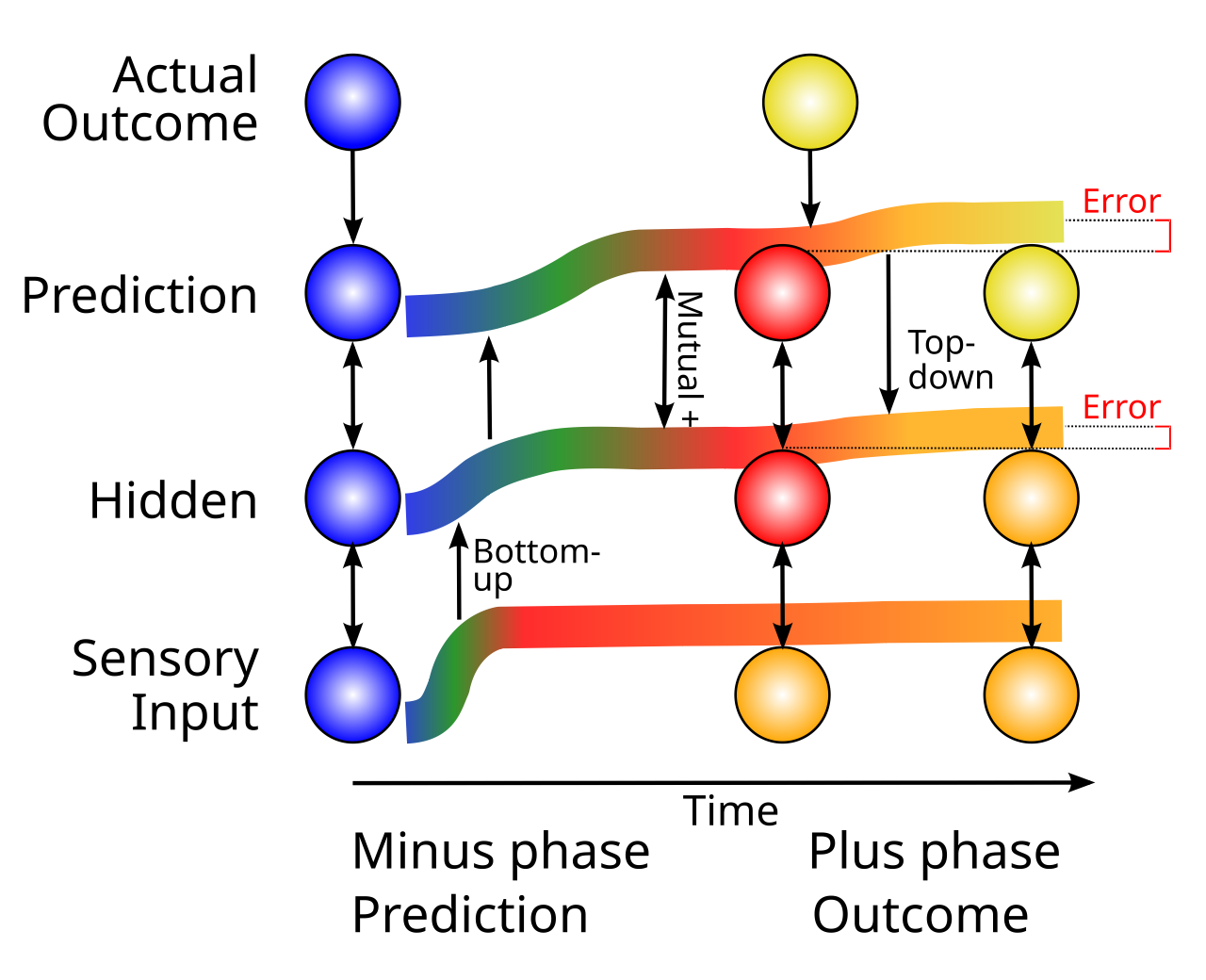
Figure 1: How bidirectional activation propagation can communicate error signals, in the simplest case of a three-layer network mapping from a Sensory Input to a Prediction output, with the Actual Outcome driving the Prediction layer only in the later plus phase, after an initial minus phase when the prediction is generated. The Error is the temporal difference between the (plus – minus) activity levels. There is just one network with three bidirectionally connected units, as shown at the left; the networks shown further to the right are snapshots of the activity state of this network at different points in time, which evolves from left to right. The thick colored lines also show the activation level of each of the three neurons over time, both in terms of the line height and the brightness and warmth of the color gradient. Initially, each neuron is inactive (blue). Then, external Sensory Input arrives, and a wave of bottom-up excitation propagates upward through the Hidden and Prediction layers. Critically, the Prediction and Hidden neurons mutually excite each other via bidirectional connections, which contributes to each of their activity levels. The snapshot of the network in the middle shows the neural activity at the end of the minus phase. Then, at the start of the plus phase, the Actual Outcome arrives, which is more active than the Prediction, and it therefore drives more activity in the Prediction neuron. This propagates top-down to the Hidden neuron as well, which is the key mechanism by which bidirectional connectivity communicates error signals, causing the Hidden neuron to have a (plus – minus) activity difference, reflecting the top-down influence from the Prediction layer. This temporal-difference based Error signal provides a good approximation to the error backpropagation error gradient (O’Reilly, 1996).
Figure 1 shows all of the major dynamics that enable bidirectional excitatory connections coupled with a temporal derivative learning mechanism to compute an error gradient. This figure is a more detailed version of the simple Minus phase \(\rightarrow\) Plus phase Figure 1 in the temporal derivative page.
The thick lines trace the activity of three representative neurons over time, in a predictive learning context where the network generates a “high activity” prediction on the Prediction layer neuron, which is contradicted by the “low activity” Actual outcome. At the start, all neurons are inactive (which is not typically the case in the neocortex, but is useful for the illustration). Then, sensory input drives activity in the Input neuron, which then excites the Hidden and Prediction neurons in turn, assuming they have strong excitatory weights between them (in a real network, there are many neurons in each layer and richer patterns of weights, etc).
The result of this initial wave of activity is a briefly stable Minus phase state of activity throughout the network, which is shown with the “snapshot” of the neurons at that point in time. This network state represents the collective prediction state of the network. Critically, the bidirectional excitatory connectivity causes the Hidden and Prediction neurons to be more excited than they would with only feedforward connections: they are mutually reinforcing each other’s activity. It is this mutual interdependence that enables bidirectional connectivity to communicate error signals.
Also, at no point is there any modulation of bottom-up vs. top-down connections or exclusive use of either one of those pathways: everything is bidirectionally interacting always. This is a key difference from structurally based error backpropagation models that require separation of bottom-up and top-down pathways (see Lillicrap et al., 2020 for a review).
The critical role of bidirectional interdependence is evident when the Plus phase arrives, which is when the Actual outcome that was being predicted actually happens, driving neural activity directly in the Prediction layer. In the case illustrated in the figure, this Actual outcome is “low activity” (blue), which contradicts the “high activity” prediction. Therefore, the Prediction layer is inhibited by this “negative” outcome, and its activity decreases. This decrease in activity then propagates down to the Hidden layer, which also becomes less active. (The actual dynamics in the brain operate over distributed patterns of activity in the context of pooled inhibition, so the difference between a prediction and an outcome is not generally about “high activity” vs. “low activity” but rather about different distributed patterns of activity, but that is more difficult to represent in a figure).
Thus, the Hidden neuron experiences a temporal derivative that reflects the corresponding temporal changes on the Prediction layer, by virtue of its bidirectional connectivity. The mathematical derivation below shows that this temporal derivative provides a good approximation to the error gradient computed by error backpropagation.
In effect, GeneRec uses activation states to compute error derivatives, while backpropagation directly computes an error gradient that is entirely separate from its activation state. As a consequence, GeneRec automatically generates optimized representations that include the error gradient in the plus phase, which is equivalent to a form of backpropagation to activations, whereas standard feedforward backpropagation networks do not, as we elaborate below. This is in addition to the existing optimization of the representations via constraint satisfaction, also driven by bidirectional connectivity.
In sum, the GeneRec algorithm shows how bidirectional connectivity, which is a prominent feature of the neocortex, enables powerful error-driven learning in a biologically plausible manner. Various closely related proposals have also been advanced since the original GeneRec paper, providing different analysis and routes of derivation (Xie & Seung, 2003; Scellier & Bengio, 2017; Whittington & Bogacz, 2017).
Approximation to backpropagation
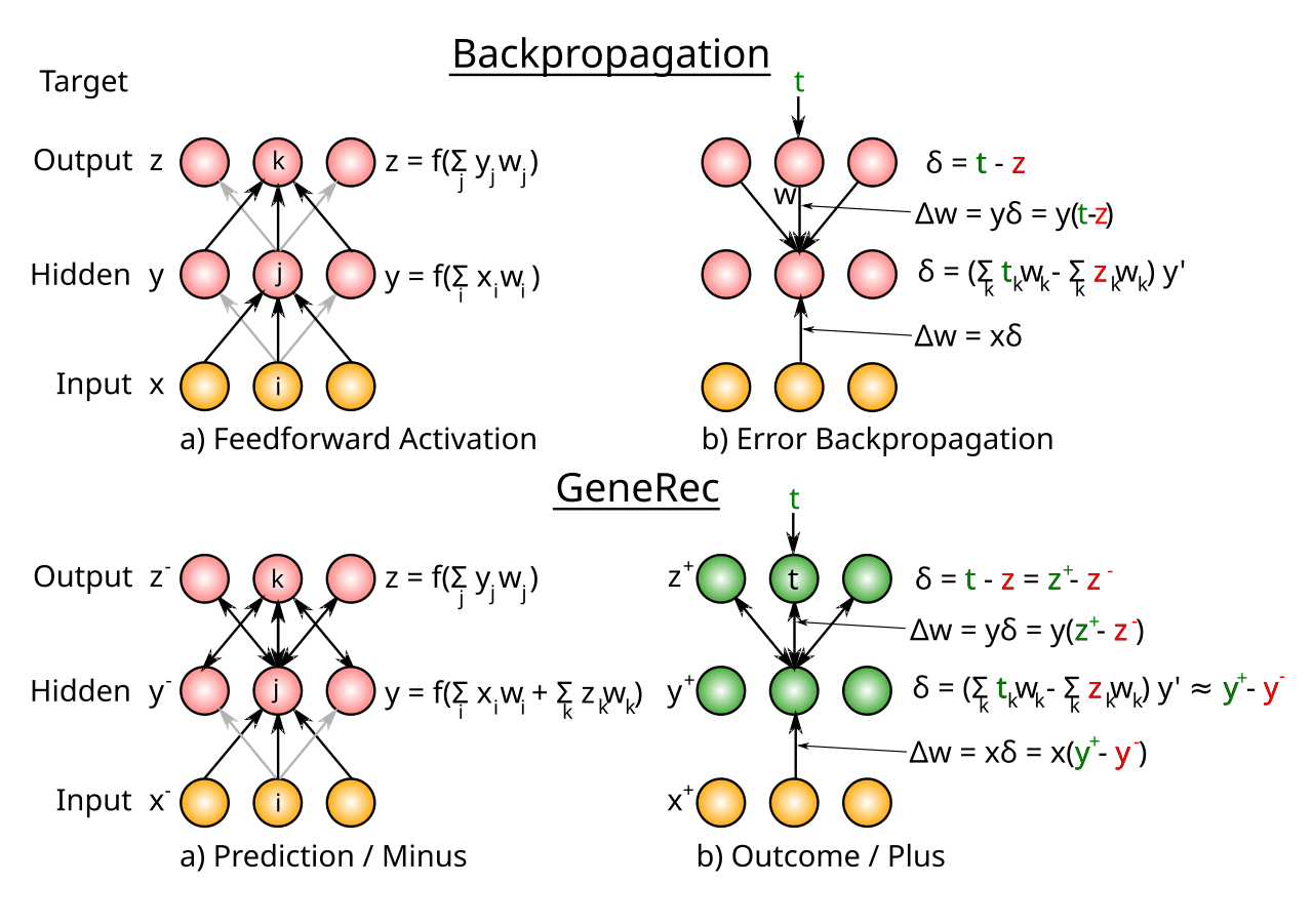
Figure 2: Illustration of GeneRec computation in three-layer network (bottom panel) in comparison to error backpropagation (top panel; explained in that page). Activations settle in the Prediction / Minus phase, in response to Input activation. Activation flows bidirectionally, so that the Hidden units are driven both by Input and Output units, as shown with the net input equation broken out separately for each). In the Outcome / Plus phase, “target” values drive the Output unit activations, and due to the bidirectional connectivity, these also influence the Hidden units in the plus phase, as emphasized in the prior figure. The δ error gradient factor from backpropagation is closely approximated by the difference in hidden unit activations between the plus and minus phases. An essential difference is emphasized by the green color in the plus phase: only in GeneRec does the neural activation change to reflect the “experience” of the plus phase outcome. In backpropagation, the target / output state is purely “virtual” and only latent in the error gradient.
Figure 2 shows how GeneRec compares with the error backpropagation algorithm (see that page for necessary background). The key result is that the \(\delta\) error gradient value from backpropagation can be closely approximated by plus \(-\) minus phase activation differences. With that approximation in place, the learning rule is the same as in backprop (\(x \delta\)), omitting the learning rate factor \(\epsilon\) for simplicity:
\[ \Delta w = x^- \delta \approx x^- \left(y^+ - y^- \right) \]
The central intuition conveyed in Figure 2 is that the \(\delta\) value in backpropagation (top panel) for the hidden unit consists of two separate net-input like sum factors, one with the output units at their target activations \(t_k\), and the other with the outputs with their “prediction” activations \(o_k\). These same factors are present naturally in a bidirectionally connected network receiving top-down projections from the output layer.
The hidden neuron is also receiving bottom-up input from the Input layer, but these are constant, so when we subtract the plus \(-\) minus phase activations, these cancel out. As an extra bonus, subtracting the two activation states implicitly computes the derivative of the activation function, which is an important component of the \(\delta\) equation.
Another critical difference emphasized in Figure 2 is that only the GeneRec network has activation states that reflect the “experience” of the outcome, in the plus phase. In the backpropagation network, the target / outcome state is only represented “virtually” in the error gradient. Given that we obviously experience the outcomes that shape our learning, this is another significant plausibility issue with error backpropagation, in addition to the optimized representations benefits from representing the outcome state as network activity.
Weight symmetry
A careful observer might have noticed that the GeneRec approximation to backpropagation depends on the top-down weights being symmetric with the bottom-up weights, so that the influence of the hidden neurons on the output can be estimated by the reciprocal pathway from output to hidden. This same kind of symmetry constraint applies to the Boltzmann machine, and to the application of overall energy functions as in the Hopfield network (Hopfield, 1995). Interestingly, Galland & Hinton (1991) found that even fairly significant levels of asymmetry in the form of missing connections between the feedforward and feedback pathways did not impair learning in a deterministic version of the Boltzmann machine.
However, that model was using a symmetric learning rule (Contrastive Hebbian Learning; CHL), whereas the GeneRec learning rule in Eq 1 is not symmetric: if you exchange x and y values, it is not the same. Interestingly, the CHL learning rule emerges from a modified version of Eq 1 that is symmetric (by adding together both directions of this equation), and that uses an average of the minus and plus phase states for the sending neuron activity. This later modification looks like this:
\[ \Delta w = \frac{1}{2} \left(x^- + x^+\right) \left(y^+ - y^- \right) \]
and O’Reilly (1996) showed that it is effectively an application of the midpoint method of numerical integration (also known as the second-order Runge-Kutta method; Press et al., 1988). Consistent with this analysis, learning is faster overall using this version of the learning rule versus Eq 1.
The idea to explore this variant arose because there are now two activation states for each sending neuron across the two phases in GeneRec, and it was not clear which one would work better. Mathematically, backprop effectively uses the minus phase state as shown in Eq 1 (because it only has minus phase activations), but the plus phase value is conceptually “more correct” because it represents the activity with the correct prediction in place. The midpoint method effectively splits the difference and takes a point half-way between the prior and “more correct” integrated value.
The combination of symmetry preservation and this midpoint method results in this equation:
\[ \Delta w = \frac{1}{2} \left[ \left(x^- + x^2\right) \left(y^+ - y^- \right) + \left(y^- + y^2\right) \left(x^+ - x^- \right) \right] \]
which simplifies to the CHL equation:
\[ \Delta w = \left(x^+ y^+\right) - \left(x^- y^- \right) \]
Remarkably, this same CHL equation can thus be derived from multiple different starting assumptions (Boltzmann machine, Movellan & McClelland, 1993), and it is an appealingly simple equation that is just the difference of two Hebbian learning factors.
Because this CHL equation is symmetric, it tends in practice to drive initially asymmetric weights toward symmetric values over time, and extensive experiments with GeneRec learning in Leabra models showed significant robustness to asymmetry in random initial weights. Therefore, this does not appear to be a major concern.
Relation to the deterministic Boltzmann machine
A GeneRec network using a simple sigmoidal logistic activation function and the above CHL learning rule is mathematically equivalent to the deterministic version of the Boltzmann machine (DBM), which was explored in a series of papers in the early 1990’s (Galland & Hinton, 1990; Galland & Hinton, 1991; Galland, 1993). This model can be derived from the original stochastic Boltzmann machine (SBM) (Ackley et al., 1985) by applying a mean field approximation, which is a standard technique in statistical physics.
It was initially thought that it might overcome some of the significant computational limitations of the SBM by avoiding the need for extensive statistical sampling, but the subsequent conclusion was that the continuous rate-code activation states caused the network to get “stuck” in attractor states that deviate significantly from the idealized thermal equilibrium that is required for the mathematical analysis of the SBM. In practice, the model failed to work well in deeper networks with multiple hidden layers.
However, extensive work with the Leabra model using a version of the CHL learning rule showed that this limitation could be overcome to some extent, by including pooled inhibition (which keeps neurons in their more linear, sensitive activation range) and a systematic reduction in the strength of top-down pathways relative to bottom-up ones, which is critical for preventing the model from “hallucinating” too much based on these top-down expectations (neuron dendrites).
Nevertheless, the fact that rate-code activations are continuously broadcasting at every time step makes them prone to developing excessively strong attractor dynamics, and the use of discrete spiking neurons in Axon has further reduced problems with learning getting stuck. In effect, discrete spiking is more similar to the stochasticity present in the original SBM model, but the additional mechanisms providing stable activation states in Axon also make it more efficient at converging on a reasonable equilibrium state than the SBM – a classic “best of both worlds” solution.
These same attractor dynamics issues also affect recurrent versions of error backpropagation networks, including the Almeida-Pineda (AP) model (Almeida, 1987; Pineda, 1988) and the more general backprop-through-time (BPTT; Werbos, 1988; Werbos, 1990), which can learn arbitrary temporal sequences. Neither of these algorithms are widely used, because they are both more computationally expensive and generally do not work very well in practice (although Liao et al., 2018 have made some improvements to the AP model). In the exploration of AP in O’Reilly (1996), it was clear that this model suffers from the same kind of excessive attractor dynamics problems as the DBM / plain GeneRec, which makes sense given the strong mathematical relationship between these algorithms.
The recent framework of Linsley et al. (2020) provides a way to parameterize learning between the more general flexibility of BPTT and the more limited attractor-dynamics of AP, and they found in practice that their models worked best on a range of sequential visual processing tasks when this parameter was very close to, but not fully at, the AP end of the spectrum. This suggests that the more constrained attractor-based learning performed by GeneRec is likely to be generally beneficial, but not entirely sufficient. Critically, the predictive learning framework used in Axon provides additional temporal context state in addition to the basic attractor dynamics imposed by bidirectional connectivity, and this constrained combination works well in practice for solving challenging sequence learning problems.
Mathematical details
For completeness, this section steps through the equations depicted in Figure 2 showing the derivation of GeneRec from error backpropagation. The key step is just the rearrangement of the expression for the \(\delta\) value on the hidden unit in backpropagation, which is:
\[ \delta_j = \left( \sum_k (t_k - z_k) w_k \right) y' \]
This sum of the error gradient on the output layer (\(t_k - z_k\)) can be rearranged into two separate sums, one with the output in state \(t_k\), and the other with \(z_k\):
\[ \delta_j = \left( \sum_k t_k w_k - \sum_k z_k w_k \right) y' \]
The key insight is then to realize that these separate factors are present in the net input to the bidirectionally connected hidden unit, in the plus and minus phases:
\[ \eta_j^+ = \sum_k t_k w_k + \sum_i x_i w_i \]
\[ \eta_j^- = \sum_k z_k w_k + \sum_i x_i w_i \]
The constant input from the Input layer cancels out in a subtraction of these terms, leaving the core of the \(\delta_j\) term:
\[ \eta_j^+ - \eta_j^- = \sum_k t_k w_k - \sum_k z_k w_k \]
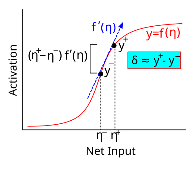
Figure 3: The slope (derivative) of a function times the difference in the inputs to that function at two different points (+ and - phases) can be approximated by the difference in the function evaluated at those two points. In effect, this difference in activation values implicitly computes the derivative of the activation function.
The final step necessary to get \(\delta_j\) is to account for the presence of the derivative of the activation function \(y'\) in Eq 6. Using the basic principles of calculus (Figure 3), we know that the difference between a function evaluated at two different points can be approximated as the difference between the two points, times the derivative of the function:
\[ f(a) - f(b) \approx f'(a) (a-b) \]
Putting this all together, we get the key GeneRec approximation for the \(\delta\) error gradient:
\[ \delta_j = \left( \sum_k t_k w_k - \sum_k z_k w_k \right) y' \approx y_j^+ - y_j^- \]
An important practical advantage of using the difference in activation states in Eq 6 is that it implicitly computes the derivative of the activation function, which avoids the need for an explicit equation for this derivative. This is critical when you consider the complexity of the biologically based activation functions used in Leabra and Axon (neuron) operating in the context of extensive pooled inhibition.