Drift diffusion

The drift-diffusion model (DDM) is an abstract, mathematically simple model of a two-alternative forced-choice (2AFC) decision that provides an optimal integration of information over time, in the sense that it gives the most accurate results in a fixed amount of time, or conversely, for a given accuracy, it gives the result in the shortest amount if time (Bogacz et al., 2006). It is a continuous version of the sequential probability ratio test (SPRT), which likewise was proven to be optimal for discrete processes (Wald, 1947; Wald & Wolfowitz, 1948).

The DDM model provides an accurate measure of human reaction time distributions (RTs) across a wide range of 2AFC tasks (Laming, 1968; Ratcliff, 1978; Stone, 1960; Ratcliff & Rouder, 1998), and neural correlates of the central accumulation process in a DDM has been identified in various brain areas (Shadlen & Newsome, 2001; Gold & Shadlen, 2002; Ding & Gold, 2013), including in the basal ganglia (Yartsev et al., 2018; Dunovan et al., 2015; Doi et al., 2020).

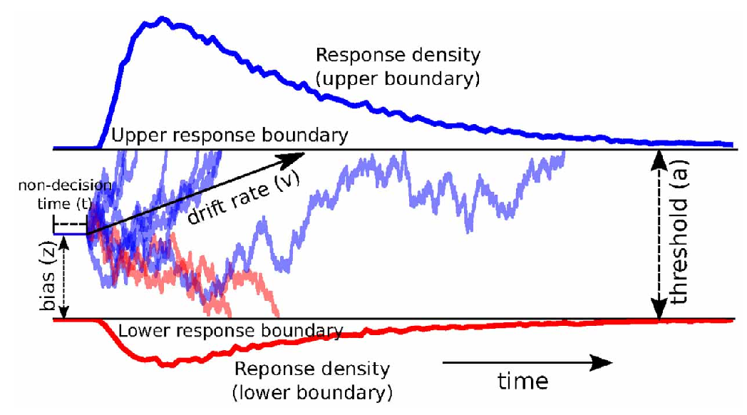
The drift-diffusion model involves an accumulation process that is driven by two force: a systematic drift that reflects the strength of an underlying signal (e.g., how clearly one perceives a stimulus) and a noise (diffusion) process. There are two bounds, upper and lower, and whenever the accumulated value crosses a bound, the decision is counted. The distribution of boundary-crossing times provides a good fit to human and animal reaction times across a wide range of studies.

Figure 1: The drift-diffusion model involves an accumulation process that is driven by two force: a systematic drift that reflects the strength of an underlying signal (e.g., how clearly one perceives a stimulus) and a noise (diffusion) process. There are two bounds, upper and lower, and whenever the accumulated value crosses a bound, the decision is counted. The distribution of boundary-crossing times provides a good fit to human and animal reaction times across a wide range of studies.

Figure 1 shows the key elements of the DDM. Typically, the drift rate is positive, with the upper boundary representing correct responses, while the lower boundary represents an error. One of the important strengths of the DDM model is that it provides a good account of the distribution of error reaction time distributions.

The DDM model has often been applied to tasks where the relevant information is weak and/or stochastic in nature, such as a display with dots moving in largely random directions, but with a given underlying probability of moving in a given target direction. This provides a good fit to the temporally extended accumulation process in the DDM. This accumulation process is also a good fit to any neural integration process over discrete spiking neurons, which are also noisy and the longer you integrate the signal, the better accuracy you’ll get.

The BG ventral simulation shows how an accumulator-like process within the basal ganglia can exhibit RT distributions similar to those of the DDM model, consistent with the evidence that this is the neural locus of a DDM-like integrator process (Yartsev et al., 2018). The mechanisms underlying this integration process are not specifically DDM-like, but perhaps the analysis of Bogacz et al. (2016) might provide some relevant insight into how it relates.