FSA simulation

This simulation demonstrates a small-scale predictive learning Axon model learning to predict sequences of tokens generated by a Finite State Automaton (FSA), as widely examined in human learning studies (Reber, 1967; Cleeremans & McClelland, 1991). The network learns the “deep structure” of the underlying grammar that generates partially ambiguous observable state tokens, strictly through errors in predicting the sequences of these tokens, and thus serves as a simple, small-scale instance of the larger predictive learning framework. The task is relatively challenging due to the ambiguities present in the surface tokens, and provides a good test of the underlying learning mechanisms.

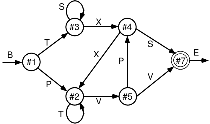
Figure 1: Finite state automaton (FSA) grammar used in implicit sequential learning exerpiments (Reber, 1967) and in early simple recurrent networks (SRNs) (Cleeremans & McClelland, 1991). It generates a sequence of letters according to the link transitioned between state nodes, with a 50% random choice for each node of which outgoing link to follow. Each letter (except for the B=begin and E=end) appears at 2 different points in the grammar, making them fully ambiguous. This combination of randomness and ambiguity makes it challenging for a learning system to infer the true underlying nature of the grammar.

Figure 1 shows the FSA grammar used. Each node has a 50% random probability of branching to two different other nodes, and the labels generated by node transitions are locally ambiguous (except for the B=begin and E=end states). Thus, integration over time and across iterations are required to infer the systematic underlying grammar. Given the random branching, accurately predicting the specific path taken is impossible, but we can score the model’s output as correct if it activates either or both of the possible branches for each state.

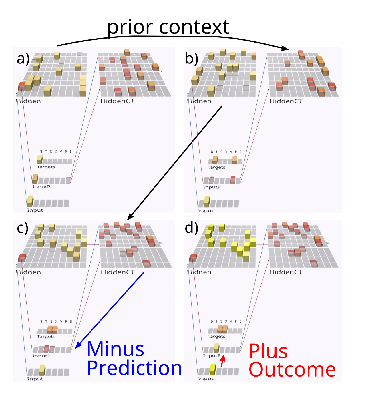
Figure 2: Predictive learning model applied to the FSA grammar shown in previous figure, showing the prediction state (end of the minus phase) for the first 3 steps of a sequence, after having learned the grammar, followed by the plus phase after the third step. The Input layer provides the 5IB drivers for the corresponding InputP pulvinar layer, and the Targets layer is purely for display, showing the two valid possible labels that could have been predicted. The model’s prediction is scored as accurate if either or both targets are activated. The HiddenCT layer drives the prediction over the pulvinar, and it receives input from the Hidden layer (superficial lamina 2-3 neurons) that reflect the previous time step’s activation state. Thus, even though the correct answer is always present on the Input layer for each step, the CT layer is nevertheless attempting to predict this Input based on the information from the prior time step. a) In the first step, the B label is unambiguous and easily predicted (based on prior E context). b) In the 2nd step, the network correctly guesses that the T label will come next, but there is a faint activation of the other P alternative, which is also activated sometimes based on prior learning history and associated minor weight tweaks. c) In the 3rd step, both S and X are equally predicted. d) In the plus phase for this trial, only the X present in the Input drives HiddenP activations, and the pathways from pulvinar back to the cortex convey both the minus-phase prediction and plus-phase actual input.

Figure 2 shows how the predictive learning mechanisms based on the thalamocortical loops through the neocortex and thalamus work in the context of the model that we’ll start exploring now. The prediction in the minus phase comes from the pathway from the HiddenCT layer, representing the deep layer 6CT neurons in the neocortex, which project to the InputP pulvinar layer, which represents the prediction in the minus phase. The actual outcome in the plus phase comes from the Input layer activity: the InputP layer has a special bit of code that grabs the activity of its corresponding driver layer, only in the plus phase (you can click on the InputP layer and see this specified there).

• • Click sim-fsa:Wts in the Network variables, and then on sim-fsa:r.Wt to view the receiving weights into neurons as you click on them in the network.

You should see the initial random weights associated with the pathways indicated by the arrows. The CT layer has recurrent self connections that allow it to better maintain information over time, so that it can leverage information from points even earlier than the prior trial.

• • Click sim-fsa:Act (category then variable) and click on sim-fsa:Step which will run one 200 ms Trial of updating.

On this very first trial, you can clearly see that the CT neurons are only activated by prior trial’s activity states, because they remain inactive on this trial. This delayed responding of the CT neurons is essential for enabling predictive learning even as the rest of the network is processing the current input information, which is being predicted.

• • To see the phase-wise differences in prediction versus outcome, select sim-fsa:Network/Stats and then sim-fsa:ActM to view the minus phase activity state. Because the minus phase prediction is generated by the CT layer, InputP is also blank. Then click on sim-fsa:ActP to see the plus phase activations, where InputP now reflects the current sensory Input.

You can continue to sim-fsa:Step through the trials, observing the sequence of inputs and the network’s predictions, which will generally be incorrect because the model has not yet learned.

• Click on sim-fsa:Train Epoch Plot to see a plot of the training error, then set the Step level to Run and click sim-fsa:Step to start training the model. When the error gets close to zero, click sim-fsa:Stop to stop the training.

• Then, you can switch back to viewing the sim-fsa:Network, and switch the Step back to Trial, and sim-fsa:Step through the sequence of inputs again. You should observe that the minus-phase predictions are now accurate.

On average, it takes roughly 60 epochs for the network to learn to a criterion of two epochs of zero errors in a row.

The primary point of this model is to test the learning capabilities of the deep predictive learning algorithm.