
Everything is Search, and Gradient Descent (in Spiking Networks) is the only Efficient Search Mechanism
By Randall C. O'Reilly
Astera Institute; Department of Psychology
Center for Neuroscience, University of California Davis
correspondence: oreilly@ucdavis.edu
June 7, 2026, Version: 1
Abstract: .
Most cognitively relevant computation can be seen as variants of a search process, providing a unified basis for understanding the essential properties of the underlying processes across different domains and timescales of such search processes. Stochastic gradient descent in suitably smooth systems is the only known solution to a search process that scales in polynomial time, in the face of exponentially large search spaces. The computational cost properties of this search process can be understood within computational complexity theory (Arora & Barak, 2009), where the class of NP hard and NP complete problems have been rigorously analyzed.
The prototypical successful example of stochastic gradient-based search in exponentially-large spaces is a neural network learning via error backpropagation to search the space of all possible representations of a given problem (Rumelhart et al., 1986; LeCun et al., 2015), which underlies current large-language models and other very large AI models (Naveed et al., 2025). The network architecture in these models is optimized in ways that make the gradient descent landscape sufficiently smooth to enable this procedure to succeed. The nature of these smoothness constraints is critical, in relation to other nearby cases that have proven less successful for gradient-descent-based search. Specifically, architectures that minimize interdependencies and have more linear response dynamics appear to be more successful.
Aside from learning representations, another important search domain involves the search for effective interpretations of the current state context (i.e., in context learning). This search process can be understood within the general framework of constraint-satisfaction search: finding the representations that optimize the various constraints from the current context, based on representations that have been shaped over the course of learning. This can also be described as the inference problem, e.g., in standard Bayesian frameworks (e.g., Kersten et al., 2004).
A prototypical example of this kind of constraint-satisfaction search is the travelling salesman problem (TSP), which involves finding the minimal distance route between a set of \(n\) randomly-distributed cities (Arora, 1998; Hopfield & Tank, 1985). In the neural network framework, such problems have been explored using bidirectionally-connected networks that perform stochastic gradient descent in activation space (e.g., Hopfield & Tank, 1985; Ackley et al., 1985).
Thus, stochastic gradient descent appears to provide a consistent overarching solution to these two intertwined forms of search, where learning provides a longer-time-scale shaping of the representations upon which the online inferential constraint-satisfaction search process operates. The empirical fact that only neural networks have proven successful for large-scale gradient-based search in learning can be leveraged to restrict the focus on such architectures for the online inferential search process.
In this context, it is notable that most neural network architectures in wide use today are strictly feedforward, and therefore do not support a gradient-descent inferential process. Instead, current LLM models for example use very deep architectures to effectively unroll the bidirectional interactions that would otherwise occur in a bidirectionally-connected network (McClelland et al., 2020), and further employ chain of thought outer-loop search processes for additional iterations, that help to converge on better representations of the current situation.
By contrast, the mammalian neocortex is extensively bidirectionally-connected, and therefore should in principle be capable of extensive online bidirectional constraint-satisfaction processing, similar to the original neural network models. In this context, we show that certain properties of biological, discrete-spiking neurons (as contrasted with continuous-valued rate-code neurons like those in most neural network models) are important for facilitating this form of stochastic gradient search. In particular, the following properties are identified:
• Compared to rate-coded networks, spiking dynamics allow graded, probabilistic information to be represented throughout the network (not just in restricted layers, such as the variational auto-encoder), and overall are much better at avoiding getting stuck in bad local minima during the gradient-descent process.
• Pervasive bidirectional connectivity allows detailed constraints in deep, modality-specific processing areas to effectively constrain more abstract interpretations generated in higher-level integrative areas, which contrasts with the loop-unrolling behavior of deep feedforward networks, which only support unidirectional flow through more abstract, higher-level areas. This may contribute to the tendency of LLM models to confabulate, for example.
• In general, a bias toward forming low dimensional final states represents an important additional constraint on the inference search process, which also favors the properties of the bidirectional neural network search process, as compared to the feedforward loop unrolling. Specifically, the bidirectional network tends to settle into discrete attractor states, whereas the loop unrolling process through feedforward layers does not have this property. This is also likely a factor in the tendency of LLM models to confabulate.
Thus, this analysis suggests that the specific properties of the mammalian neocortex could be particularly well-suited for this inferential online search process, for finding sensible low-dimensional interpretations of the environment, that then provide a suitable basis for acting in the world. Given that the motor action space is necessarily low-dimensional, the ability to rapidly compress the high-dimensional environmental state into appropriate low-dimensional interpretations likely has significant survival benefits (Sridhar et al., 2021).
Furthermore, the interplay of bidirectional (recurrent) processing and low-dimensional activity states may have deep connections to the nature of human consciousness, given the prominent role that these features play in most neuroscience-based theories (e.g., Lamme, 2006; Tononi & Koch, 2015).
Search is universal
Every cognitively relevant type of computation can be cast as form of search:
• Problem solving can be defined as search through problem space, as in many classical symbolic artificial intelligence (AI) systems (Newell & Simon, 1972; Newell, 1990).
• Planning is search through action space to accomplish a desired outcome, which is the focus of many approaches in model-based reinforcement learning.
• Learning is search through representation space, to find the best basis space for representing inputs, that supports the desired computational processes and behavioral outputs.
• Inference is search through learned representations to find the best interpretation of a given input stimulus relative to the stable semantics of the environment.
• Evolution is search through phenotype space, e.g., as in genetic algorithms.
This is not an empty tautology, because it provides a unified understanding about the central problem faced in all of these domains: Each of these search spaces is plagued by the curse of dimensionality, and effective solutions for real-world, large-scale problems must somehow tackle the exponential explosion problem.
Indeed, the field of computational complexity provides a unified framework based directly on the process of search, that formally quantifies the computational cost of different types of problems using universal Turing machines (Arora & Barak, 2009). The core distinction here is in terms of polynomial (P) versus exponential time costs, where polynomial means that the compute time is on the order of (expressed as \(O(f(n))\)) a constant exponential factor of the dimensionality of the problem space (e.g., \(O(n^2)\) where the polynomial factor is 2). By contrast, exponential time means that \(n\) is instead in the exponent, e.g., \(O(2^n)\), which is where the exponential explosion problem occurs as \(n\) increases, making these problems intractable.
Computational complexity theory defines an equivalence class across a wide range of problems, known as NP complete, where NP stands for nondeterministic polynomial time. The terminology is not particularly intuitive, but the NP complete class defines a large set of decision problems that require exhaustive, enumerative (i.e, brute force) search over an exponentially-large space of possible solutions, where each decision evaluates a binary (yes or no) function, which itself runs in polynomial time (which accounts for the P in NP).
Formally, the NP class is defined in terms of a nondeterministic Turing machine (which is where the N in NP comes from) which effectively performs a brute-force search process over a space of deterministic Turing machines, each of which runs its evaluation function in polynomial time. The more general NP hard designation is not restricted to binary decision problems – the complete equivalence class only applies to such problems that can all be reduced to being effectively notational variants of each other. Most cognitively relevant computations such as Bayesian inference and optimal decision making are at least in the NP-hard class (Rooij et al., 2012).
The framing of computational problems as search provides a crucial, intuitive insight into why some problems are exponentially costly, and others are not. In effect, if there is no efficient way to narrow the search space, then there is no other alternative to performing the brute force search through all possible states. If there were an efficient, systematic way to narrow the search process, then it could potentially move from the NP complete class to the tractable P class.
An illustrative case is the classic travelling salesman problem (TSP), which involves finding the minimal distance route between a set of \(n\) randomly-distributed cities, which is in the NP complete class. However, TSP can be solved in polynomial time if there is an underlying metric space (e.g., Euclidean distances) and the optimality constraint is relaxed, so that a solution only need be within some factor of the shortest distance of a route between the given cities (Arora, 1998). Interestingly, either of these constraints alone is insufficient. The resulting algorithm indeed involves an efficient way of narrowing the search space by dividing it into different subregions and applying a novel search constraint on those regions.
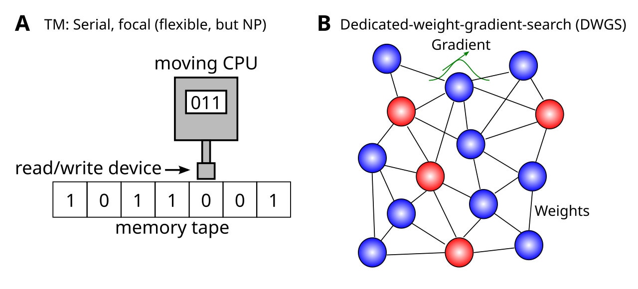
Figure 1: The two main computational frameworks for understanding the computational complexity of search as a general computational process. A In a Turing Machine, TM, there is a single focus of computational processing at each point in time, which can involve one of a small set of finite operations (read / write from a long-term “tape” storage, or operations on elements in active memory). If there is no way to systematically narrow the search space, it must serially enumerate all relevant combinations to find the best solution, resulting in combinatorially exponential (i.e., NP) worst-case behavior (e.g., the target ends up being the last combination considered, like finding a needle in a haystack). B In a dedicated-weight-gradient-search (DWGS) algorithm like a neural network, each unit is dedicated to a specific feature value, and synaptic weights capture all interactions. One update iteration involves gradient computations across all such units, which effectively incorporates all of the different weighted contstraints simultaneously, in choosing the next direction to search. The graded, smooth nature of the search space is essential for these incremental steps to provide an efficient narrowing of the search space. Under such conditions, a tractably small number of iterations will generally produce reasonable search results.
In this context, we can understand the stochastic gradient descent procedure in neural network models (e.g., Rumelhart et al., 1986) as a uniquely powerful way of searching exponentially-large combinatorial feature spaces (Figure 1), because the gradient-descent process provides a highly efficient way of shaping the direction of the search process toward more optimal solutions. As in the TSP problem, the success of this gradient descent procedure depends on operating within a system and environment that has some kind of underlying metric properties within a space that is fundamentally smooth enough, such that incremental graded steps are able to accumulate over iterations, and move ultimately toward a search solution. Furthermore, this process can only produce local minima in the relevant optimization metric, i.e., approximately-optimal solutions, not the absolute global optimal solution.
These key differences from the standard NP-complete version of the search process, plus the basic limitations imposed by the neural network formalism itself, ensure that gradient descent in neural networks does not provide the long-sought example of an NP-complete problem that can be solved in polynomial time (i.e., proving that NP = P). This is the same logic for why Arora (1998) also does not prove that NP = P. Nevertheless, in the real world, we are much more interested in the empirical capabilities of algorithms on large-scale problems of practical relevance, where there is no doubt of the relevance.
The success of extremely large (billions of parameters) neural-network based artificial-intelligence (AI) models depends entirely on the efficacy of this gradient-descent process. The importance of this efficient search process can also be seen in the negative case, in terms of the inability to scale up earlier symbolic AI models, for which a smooth metric gradient is undefined: symbols and the propositional structures in which they are used have discrete, “sharp” edges and many discontinuities. Furthermore, although the variational inference procedure enables gradient descent to be used on probabilistic (e.g., Bayesian) models (Blei et al., 2017), there are still limitations in such models that prevent the kind of deep scaling possible in simpler, more linear neural network models.
It is also critical to emphasize the no free lunch proscription against a generally optimal learning algorithm (Vapnik & Chervonenkis, 1971; Geman & Geman, 1984): gradient descent only works when gradients are actually useful for search, which represents a kind of bias in the algorithm, that can easily be violated and thus result in very bad performance. Empirically, it is nevertheless evident that gradient descent in neural networks is effective for a wide range of relevant problems, and recent work is making progress analyzing why this is so (Lee et al., 2019; Dauphin et al., 2014; Nakkiran et al., 2021; Shwartz-Ziv & Tishby, 2017; Vidal et al., 2017).
In the context of a neural network, the gradient-descent search process can operate on two different variables, which correspond to different effective timescales of search:
• Weights: (i.e., learning) as in the error backpropagation algorithm, which configures weights to shape the internal representations of the network over the course of many learning trials to optimize the overall objective function. In modern AI models, the objective is often the ability to predict the next element in a sequence.
• Activations (i.e., inference) within an individual learning trial, which also contributes at least in part to various types of search listed at the outset, including planning and problem-solving. This can be performed using backpropagation to activation states, or via a constraint satisfaction settling process as in the original Hopfield network or Boltzmann Machine (Hopfield, 1982; Hopfield & Tank, 1985; Ackley et al., 1985).
This more rapid time scale of search process is not typically used in current large AI models, which are based on strictly feedforward architectures that do not support this form of search. Instead, this functionality is captured in part by the attention mechanism in transformers (Vaswani et al., 2017) and cascading effects across multiple deep layers (McClelland et al., 2020). Nevertheless, it is likely that this inner-loop of constraint satisfaction search is critical for human intelligence, and, interestingly, many theories of consciousness involve a central element of this kind of recurrent, interactive processing (e.g., Lamme, 2006; Tononi & Koch, 2015).
In summary, the main point of this paper is simply to provide the broad conceptual framework articulated above, with the empirically-backed conclusion that stochastic gradient descent in weighted neural-network architectures may represent a uniquely powerful form of search, which can be seen as the central process involved in all major cognitive functions. This perspective also highlights the potential importance of the shorter time scale constraint-satisfaction search process to support inference, planning and problem-solving, which is missing in current large-scale AI models.
In the remaining sections, current research on gradient descent in learning and constraint satisfaction processing is reviewed, including new experimental results that point to important benefits of biologically-based neural network properties, including discrete spiking, surround inhibition, and the restriction to positive-only weights and activation states.
The unreasonable efficacy of gradient descent
The gradient descent procedure used in error backpropagation represents a straightforward application of the chain rule, which is part of the basic toolkit of elementary calculus, as many students learn in high school. Therefore, it does not represent any kind of advance at the basic mathematical level, as emphasized by the historical treatment of the field by Schmidhuber (2025), which cites Godfried Liebnitz (1676) as the earliest person to “discover” backpropagation, followed by a long list of other uses of similar procedures in statistical models. However, as Schmidhuber (2008) himself earlier noted, it is the last inventor that, by definition, has taken the credit, and in this case that is clearly Rumelhart et al. (1986), who went on to systematically articulate the computational advantages of this learning mechanism within a comprehensive framework that represented a paradigm shift across multiple fields.
Part of the reason that this gradient descent procedure was multiply reinvented in the context of neural network models (e.g., Werbos, 1974) is that nobody with experience in the use of this simple algorithm thought it would be successful, including Hinton and Rumelhart (Anderson & Rosenfeld, 2000). This is because there is too much risk of this procedure getting stuck in suboptimal local minima. We now understand more about why it does not generally suffer from this problem, in ways that also help to recognize that the remarkable success of gradient descent in neural networks is not likely to generalize to other contexts. Thus, there is something special about this combination of gradient descent and neural network models, and the environments upon which they’ve generally been applied.
One line of analysis has shown that instead of local minimal, most critical points in a neural network are likely to be saddle points (Dauphin et al., 2014), but in fact these saddle points are almost always avoided by first-order gradient descent methods (Lee et al., 2019). Furthermore, the final convergence states tend to be near global optima (Choromanska et al., 2015).
A number of related results point to the broader conclusion that neural networks operate largely like linear systems (Saxe et al., 2013), despite the critical presence of a nonlinearity in their activation functions, which is necessary to obtain any benefit from multiple cascaded (“deep”) layers. Indeed, the widespread adoption of the rectified linear activation function (ReLU) makes these models even closer to the linear limit, although its benefits may be more associated with its wide dynamic range and the elimination of the vanishing gradient problem.
As the size and depth of a neural network is increased, learning speed improves as roughly a power law (Bahri et al., 2024; Kaplan et al., 2020), and, counterintuitively, generalization also improves (Nakkiran et al., 2021). One important cause of these effects is the ability of larger models to more faithfully capture the statistical structure of their inputs early in the training phase, so that all of the relevant signal is retained and available for then mapping onto the relevant output patterns (Shwartz-Ziv & Tishby, 2017).
Intuitively, it seems that the central limit theorem effects (i.e., the “law of large numbers”) cause these large models to have less variance in their behavior as a result of incremental weight changes, which then allows gradient changes to have a smooth, cumulative effect, even with the stochastic sampling effects of training on small batches of training items. By contrast, weight changes in smaller networks can have more dramatic effects on network behavior, making the gradient surface rougher.
Weights vs configuration space
The formal computational complexity framework is based on enumerative and exhaustive search, which means that all possible combinations of the different elements in the space are considered (e.g., all possible routes through the cities, in the TSP problem). By analogy with an analogous situation in quantum physics, we can refer to this enumerative and exhaustive space as configuration space: the space of all possible configurations of a set of elements. The serial, computationally universal Turing machine framework has no difficulty with expressing the processing of configuration space.
However, the use of synapse-like weight parameters in neural networks represents a massive simplification of the search space relative to configuration space, because in most standard neural network models, the weights are used to compute a linear sum of weighted inputs, which imposes significant restrictions relative to any possible logical function that could be computed. While it is true that an entire multilayer neural network is a universal function approximator (Hornik et al., 1989; Schäfer & Zimmermann, 2006), that does not mean that each individual neuron can be trained to compute any function on its inputs.
Furthermore, as noted above, the success of the gradient descent search process depends on the quasi-linear properties of individual neurons, so introducing more complex functional forms within individual neurons runs the risk of negating the entire advantage of the neural network framework in the first place. Indeed, research on neurons with multiplicative elements shows that a range of non-gradient-descent based optimization techniques are required, and it is unclear what the scaling properties of these networks are (Swapna Rekha et al., 2020; Gao et al., 2019). This is a potentially important source of caution relative to the widespread interest in the advanced computational capabilities provided by active channel properties within dendritic arbors ((Hausser & Mel, 2003; Migliore et al., 1999; Poirazi et al., 2003; Jarsky et al., 2005; Spruston, 2008; Poirazi & Papoutsi, 2020).
Thus, it appears that the representational limitations of standard quasi-linear weighted neural networks are important to their success, and again we fall back on the empirical evidence that despite these limitations, such models have proven their value on a range of important real-world problems, that generally fall within the scope of the kinds of functionality present in the mammalian neocortex (e.g., visual object recognition, language prediction).
Beneficial biological constraints on constraint satisfaction search
The final contribution of this paper is to explore the potential impact of a set of biologically motivated constraints on the constraint satisfaction search through activation space, in the context of the widely-studied traveling salesman problem (TSP). We compare three models: The original Hopfield network (as in Hopfield & Tank, 1985), a mean-field, rate-coded version of that model, and a network with biophysically-based spiking neurons that are used in the Axon model, based on the adaptive exponential (AdEx) conductance-based neuron (Brette & Gerstner, 2005).
Acknowledgments
This work has benefited significantly from input from Alex Petrov and other members of the analogy discussion group, hosted by Jonathan Cohen at Princeton.
Environment desiderata
Key property is that top-down influences resolution of lower-level features. But you don’t want to hallucinate. Therefore, it should be attentional, in terms of guiding what features are relevant to resolve, and providing specific disambiguating context.
Navigation
• In general want a good synthetic model of parietal / RSC etc spatial reps for navigation.
• Each border / depth feature provides constraints on overall topology of env, collective set mutually informative for overall shape.
• Prediction is what happens when you turn: what depth map do you expect to see. Constraint satisfaction fills that in based on higher level schematic representation.
• Existing data from El-GabyHarrisWhittingtonEtAl24 and MaeleVerbelenGeorgeEtAl26 on simple 3x3 room with different sequences: higher-level rep is sequence, lower is specific view. Plan-level is how to move. Can build in motivation etc factors and just focus on the predictive learning and planning. use BG Dorsal for RL-based learning.
• Provides direct plug-in for cerebellar factor, but can build in head direction signal and visual motion signals straight away.
• Build-in detailed motion map instead of any parallax-based depth – that is the most relevant for rodent vision
Artificial synthetic env
Low-level modality inputs:
- • Each individual input feature is ambiguous
- • Feature combinations are meaningful
- • Relevant categories are low dimensional: many inputs to one category
- • This allows for incomplete inputs, can fill in missing pieces from regularities
- • multiple low-level features that could be filled-in: high-level determines what is relevant!
params:
- • N features, K values per feature
- • LC lower categories (LC << K^N)
- • Each LC defined by: M subset of features, at L-H range of values per feature. O < M features actually presented at any given time. Each
- • HC higher categories
- • same parameterization, but different instances
High-level categories:
- • Depend on different combinations of low-level features
- • So filling-in at lower level resolves higher-level
Semantic example:
- • top level: want water + absence of predator
- • low level: river bank, trees -> water (but river bank, rocks -> no water);
- • lack of odors, prey tracks (but lack of odors, predator tracks -> predator) -> no predator